In this page you will find the plots and table that I would like to include in a talk at Nançay (11/21/2011-11/24/2011) waiting for approval. Link to the website page : http://www.obs-nancay.fr/mode2011/
HESS J1857+026
The first part of the talk deal with HESS J1857+026 (https://confluence.slac.stanford.edu/pages/viewpage.action?pageId=108695188 , https://confluence.slac.stanford.edu/pages/viewpage.action?pageId=100515585). Here are the plots I would like to show :
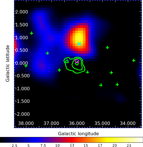
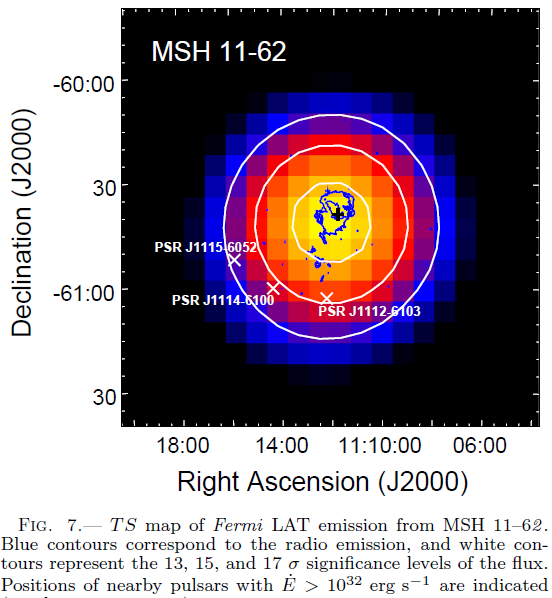
Fig. 1. TS maps computed by pointlike. The green crosses represent the sources of the 2FGL catalog included in the model. Whereas the blue X
represents the source we added in the model. The green contours represent the HESS data (Aharonian et al., 2008). The magenta circle represents
the position of PSR J1856+0245. TS map obtained between 0.1 and 1.3 GeV. This figure shows the residual
excess taken into account in our model (cyan cross).
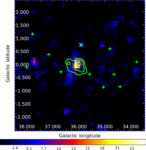
Fig. 2. TS maps computed by pointlike. The green crosses represent the sources of the 2FGL catalog included in the model. Whereas the blue X
represents the source we added in the model. The green contours represent the HESS data (Aharonian et al., 2008). The magenta circle represents
the position of PSR J1856+0245. TS map obtained between 10 and 300 GeV. The position of the Fermi excess is consistent with that of
HESS. Note that HESS J1857+026 is not included in the model.
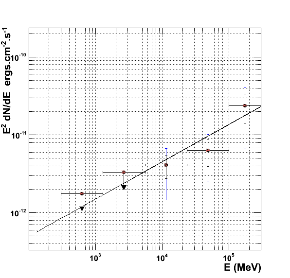
Fig. 3. LAT spectral points obtained using gtlike. The black and blue error bars corresponds respectively to the statistical and systematic error bars. The black line correspond to the best fit obtained using gtlike.
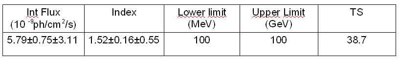
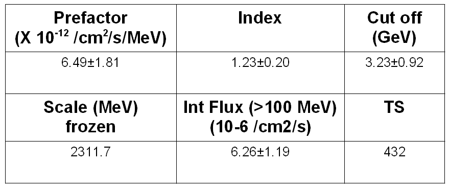
Tab. 1. Best fit parameters obtained using gtlike.
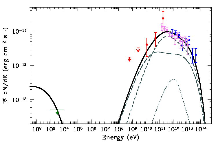
Fig. 4. Spectral energy distribution of HESS J1857+026 with a a relativistic Maxwellian plus power-law electron spectrum. The X-ray flux upper
limit obtained using Chandra(green), LAT spectral points (red), MAGIC points (violet) (Klepser et al. 2011), and H.E.S.S. points (blue) (Aharonian
et al. 2008) are shown. The black line denotes the total synchrotron, inverse Compton and pion decay emission from the nebula.Thin curves indicate
the Compton components from scattering on the CMB (long-dashed), IR (medium-dashed), and stellar (dotted) photons.
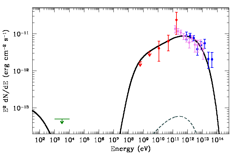
Fig. 5. Spectral energy distribution of HESS J1857+026 with an exponentially cuto power-law proton spectrum. The X-ray flux upper
limit obtained using Chandra(green), LAT spectral points (red), MAGIC points (violet) (Klepser et al. 2011), and H.E.S.S. points (blue) (Aharonian
et al. 2008) are shown. The black line denotes the total synchrotron, inverse Compton and pion decay emission from the nebula.Thin curves indicate
the Compton components from scattering on the CMB (long-dashed), IR (medium-dashed), and stellar (dotted) photons.
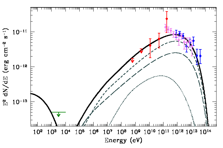
Fig. 6. Spectral energy distribution of HESS J1857+026 with a simple exponentially cuto power-law electron spectrum. The X-ray flux upper
limit obtained using Chandra(green), LAT spectral points (red), MAGIC points (violet) (Klepser et al. 2011), and H.E.S.S. points (blue) (Aharonian
et al. 2008) are shown. The black line denotes the total synchrotron, inverse Compton and pion decay emission from the nebula.Thin curves indicate
the Compton components from scattering on the CMB (long-dashed), IR (medium-dashed), and stellar (dotted) photons.
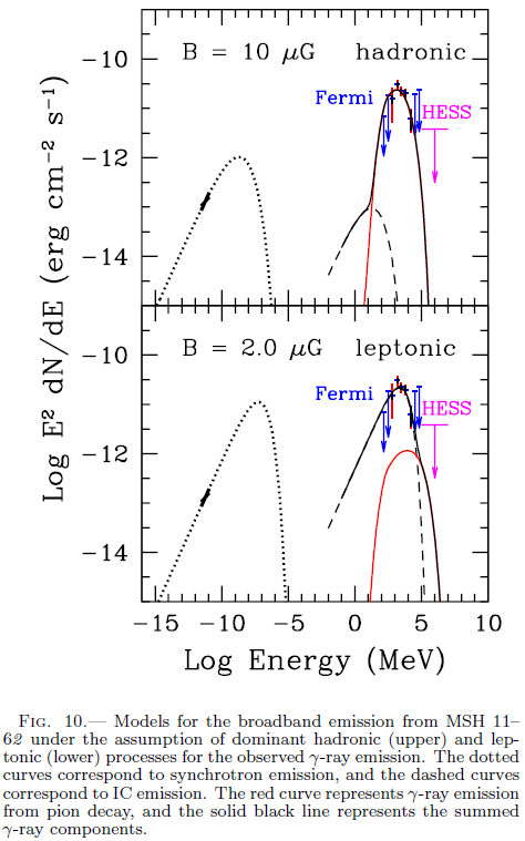
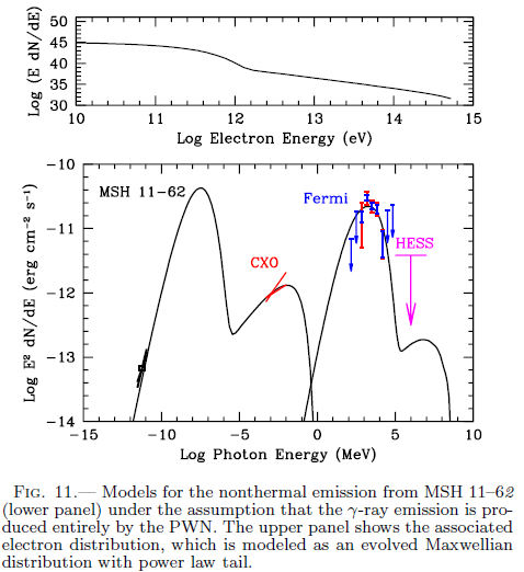
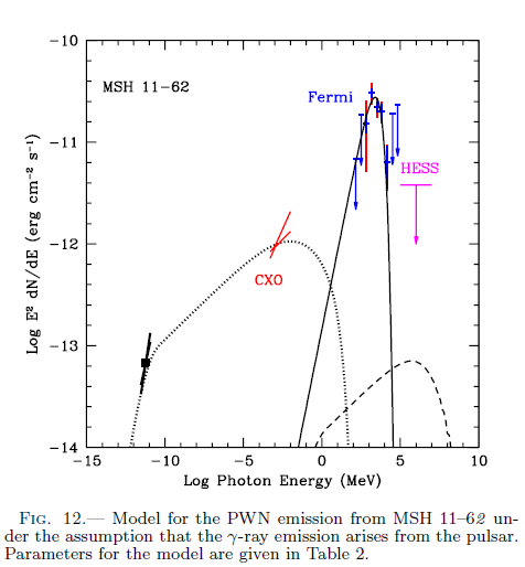
MSH 11-62
The second part deal with MSH 11-62 : https://confluence.slac.stanford.edu/display/Glast/MSH+11-62. Here are the plots I would like to show :
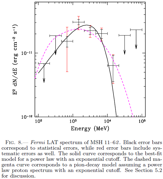
Tab. 1 . Best fit parameters obtained using gtlike for MSH 11-62. The errors correspond to both statistical and systematics added in quadrature.