HESS J1857+026

• LAT Publication and Presentation Guidelines

=Task completed
= To do

*Presentation of the LAT data analysis to the group.

LAT Contact Authors:

Other LAT Contributors:

External Authors (Requirements: SG Coord Approval,Pub-board Approval)

Agenda of the day

• Standards for High Level Analisys
• LAT Statistics Board
• Interactive LAT Source Catalog
• Analysis Users forum
• LAT Analysis Page (Workbook)

General Information (this is just an example, please update it)

Source list (if applicable)

Spatial and Spectral Analysis

The whole analysis is summarized here https://confluence.slac.stanford.edu/pages/viewpage.action?pageId=100515585.

HESS data has shown an emission located at RA=284.3°, DEC=2.68°. It remained unidentified untill the detection of PSR J1856+026 in Arecibo PALFA survey (Hessels et al 2008).

Here we tested the source for extension using pointlike then gtlike and found no significant extension.

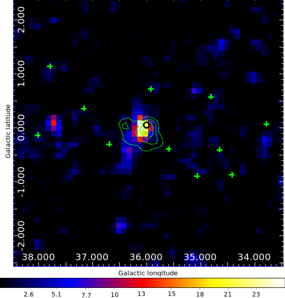
Fig. 1 Residual TS map obtained between 10GeV and 300GeV. Here HESS J1857 is not included in the model.

The green contours are those obtained using HESS data (Aharonian et al.,2008).

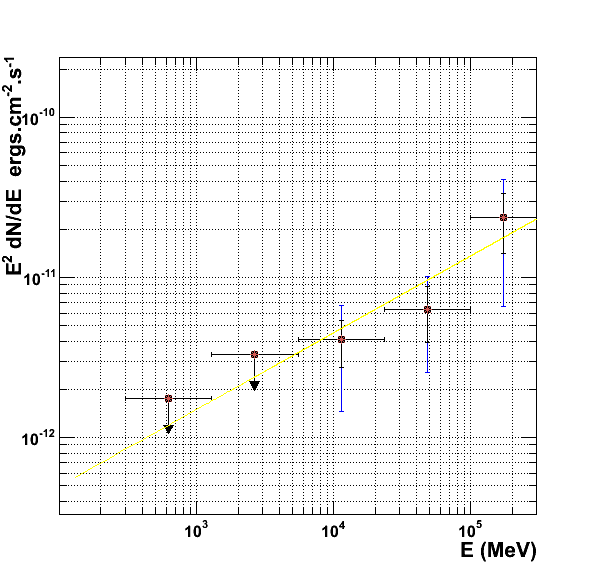
The SED shown a hard spectrum consistent with those of HESS and MAGIC. The best fit between 300MeV and 300GeV yields to the following parameters :

Int Flux(100MeV-100GeV) =  (5.79 ± 0.75 ± 3.11) X 10^{-9} MeV/cm^2/s

Gamma = 1.52 ± 0.16 ± 0.55

With a TS of 38.7.

Systematic Errors Analysis

The systematics were estimated using the bracketting IRFS, fitting the source galactic background level at +/- 6% of the value of the best fit and the systematics on the shape of the source were computed using a template consistent with the extension derived using HESS data.

Broad-Band modelling

Other Analysis

HESS 1857 is powered by a young and energetic pulsar, with a gamma-ray efficiency of 3.7% consistent with those observed using HESS data (3.1%) and consistent with the other values observed for the PWNe detected by Fermi.

An upper limit on the DC emission pulsar yield to a luminosity < 7.47 X 10^34 erg/s.

• LAT Publication Board

30/01/2012:

• draft_paper_HESS_J1857.pdfdraft (draft including the corrections in bold)
• letter to the editor

Pub. board page

Figures

Tables

Internal referee report 1 (A. Caliandro)

It is important to describe the shape and the size of the ROI.

In section 3.2 you write that sources for the xml model are extracted in a region of 10deg around HESS J1857. I guess you used the same ROI for the data selection. If it is the case (that you used 10deg ROI for the data selection) I suggest to use for the xml model a larger extraction radius (for example 15deg). In this way you avoid possible issues at the borders of your region, and the diffuse emission will be better constrained. Plausibly, this will lead to a TS value for your source slightly higher.

To evaluate the systematics due to the Galactic diffuse emission, you chnge the normalization by +-6%. This is fine, but 6% refers to the uncertainty of the model we used with P6V3. The new model you are using to analyze P7V6 data most probably and hopefully is better than the previous one.

So the systematics you evaluated are over-estimated. YOu ´can have a feeling on how large is the over-estimation comparing the systematics due to the diffuse with those due to IRFS.

Sincerely, I do not know whether a study equivalent to those performed for W51C and W49 is already done for the new Galactic diffuse model.

Since this paper is a CatII, I do not think that this kind of work should be included in it. But in the text should be clarify what I wrote above.

Anyway, this is a general problem that we should discuss within the collaboration, involving the diffuse group.

#------------------------------------------------------------------------------------------------#

I will comment section by section here below.

-- Introduction.

I found quite confusing the third paragraph of the introduction (L36)

In particular the period:

In such sources, TeV radiation can be ex-

plained by Inverse Compton (IC) scattering of an old population of leptons produced earlier in the pulsar’s life on ambient photon ?lds (CMB, IR, ...) or by ? decay from the interaction of accelerated hadrons with nuclei of the interstellar medium.

What do you mean exactly with 'an old population of leptons'?

Then, in the first paragraph you say that 'The dissipation of the rotational energy of a pulsar leads to the creation of a relativistic wind made of electron/positron pairs.'.

So why you expect pi0 decay in PWN? Maybe a more detailed explanation, and some reference will improve.

-- Timing analysis

This is a request mainly for the radio people. It is possible to evaluate the significance of the last frequency derivative in the ephemeris?

In other words, how much the fourth derivative improve the fit respect to a fit with just three derivatives?

 
-- Spatial and spectral analysis

For the description of the diffuse models you could also reference the 2FGL paper.

The description of pointlike is quite poor. Further also gtlike is used in binned mode here (I guess). I would avoid to enter in the details of the pointlike description in tis paper. I suggest to just state that pointlike is optimized for the search of the extension of a source, while it is not the case for gtlike. I would cite also the paper in preparation about search for spatially extended sources, in addition to Kerr 2011.

-- Shape and position of the source

Since you finisc the previous chapter talking about the refitting of W44, to avoid confusion I would rename this one as ' Shape and position of the HESS J1857 counterpart'

Since you cite Fig1 (b) as first, I would exchange the positions of the maps, so that the TSmap for E>10GeV is in panel (a).

The TSmap for E>10GeV is not a residual map, as you write in the caption. Otherwise we should see no source, but just statistical fluctuations.

 The ellipse errors on the localization of the source should be specified. you state that the localization is consistent with the position found in HESS. What about the consistency with the position of the radio pulsar?

-- Spectral analysis

I already commented on the systematic uncertainties.

The analysis concerning the evaluation of the pulsar DC emission (described in the last paragraph) is a little bit tricky. I ask here the same question than above. Is the radio position of the pulsar compatible with the pointlike localization? If so, you can not disentangle the pulsar DC emission from the PWN emission.

Authors response to referee 1

*"It is important to describe the shape and the size of the ROI.*

*In section 3.2 you write that sources for the xml model are extracted in a region of 10deg around HESS J1857. I guess you used the same ROI for the data selection. If it is the case (that you used 10deg ROI for the data selection) I suggest to use for the xml model a larger extraction radius (for example 15deg). In this way you avoid possible issues at the borders of your region, and the diffuse emission will be better constrained. Plausibly, this will lead to a TS value for your source slightly higher."*

This is a typo, we used a 15° extraction region to build the model. We fixed it in the text.

"

*I found quite confusing the third paragraph of the introduction (L36)*

*In particular the period:* *In such sources, TeV radiation can be explained by Inverse Compton (IC) scattering of an old population of leptons produced earlier in the pulsar’s life on ambient photon ?lds (CMB, IR, ...) or by ?decay from the interaction of accelerated hadrons with nuclei of the interstellar medium.* *What do you mean exactly with 'an old population of leptons'?* *Then, in the first paragraph you say that 'The dissipation of the rotational energy of a pulsar leads to the creation of a relativistic wind made of electron/positron pairs.'. ** **So why you expect pi0 decay in PWN? Maybe a more detailed explanation, and some reference will improve."

We removed these part of the text in the new version to be able to fit in the 4-page limit of A&A letters.

*-- Timing analysis*

*This is a request mainly for the radio people. It is possible to evaluate the significance of the last frequency derivative in the ephemeris?* *In other words, how much the fourth derivative improve the fit respect to a fit with just three derivatives?*
 

By including a fourth derivative the RMS of the timing residuals decreases in a bout 30%.
It goes from 1551.106 us  to  1081.297 us, which is equivalent to a decrease from 19 to 13 milliperiods.
The reduced chi-square of the fit also decreases significantly, changing from 22 to 5.

Even though they have no physical meaning, the use of higher order derivatives helps to flat the residuals,
allowing a more accurate folding of the gamma-ray photons on the rotational period.

*The ellipse errors on the localization of the source should be specified. you state that the localization is consistent with the position found in HESS. What about the consistency with the position of the radio pulsar?*

We added the average error on the position.

*Is the radio position of the pulsar compatible with the pointlike localization? If so, you can not disentangle the pulsar DC emission from the PWN emission.*

The radio position of the pulsar is consistent with those of the GeV source. Nevertheless, it is clear that the hard spectrum that we obtain at very high energy does not ressemble the one of a pulsar. Then, to prevent any contamination of the upper limit on the pulsar by the PWN, we added the PWN best fit parameters in our source model. This way, we can be sure that the derived upper limit is robust (as was previously done for HESS J1825).

internal referee report 2 (Andrea)

Keywords: delete 'Plerion'. It is here just a synonymous of PWN

Fermi-LAT: Fermi should be written in Italic all over the text

#--- Introduction ---#

'Recently, MAGIC reported a measured extension in the
0.2--1 TeV energy range significantly higher than the extension
reported by H.E.S.S. at higher energies (Klepser et al. 2011).'

significantly higher --> significantly larger

report here in parentheses how large is the MAGIC detection

'than the extension reported by H.E.S.S. at higher energies'
For a better comparison would be useful to declare here or in the previous paragraph the HESS energy range.

'This might support the idea that low energy electrons from the
PWN create the gamma-ray signal after diffusing away from the pulsar.'
As it is, this phrase is not easily understandable. You could spend more words to better explain this idea, or you could simply skip it. Furthermore it is not discussed in section 5.

#--- Section 2 ---#

'10 x 10 deg square around the position of HESS J1857+026.'
add here: 'aligned with celestial/galactic coordinates'

'‘Source’ events which correspond to a compromise between the
number of selected photons and the background rate.'

I would change with: '‘Source’ events which correspond to the best compromise between the number of selected photons and the charged particle residual background for the study of point-like or little extended sources'

#--- Section 3.1 ---#
You gave me a good explanation of the comment I did on the derivatives in the ephemeris of the pulsar. Why you do not add the first part of your answer in the paper? I report it here:

By including a fourth derivative the RMS of the timing residuals decreases in about 30%. It goes from 1551.106 us  to  1081.297 us, which is equivalent to a decrease from 19 to 13 milliperiods. The reduced chi-square of the fit also decreases significantly, changing from 22 to 5.

#--- Section 3.2 ---#
I think that this part still need a review.
A lot of space in this section is dedicated to the description of gtlike and pointlike, but this description is not satisfactory for a reader that is not already familiar with these tools or more generally with the maximum likelihood. Since this is a letter, I suggest to limit the description just writing that gtlike is the official tool released by the collaboration to perform the binned maximum-likelihood analysis, while pointlike is an alternative tool optimized especially for the search of the extension of a source.

The version of the ScienceTools should be cited in this section.

In contrast, I suggest to focus mainly on a more clear description of the xml model.
There should be specified:
-- the model of the galactic diffuse emission            
-- the model of the isotropic emission               
-- How many sources from the 2FGL are in your model       
-- How many sources have free parameters       
-- Which parameters of the nearby sources are free? All their spectral parameters, or just the normalization factor?

Concerning the analysis of SNR W44, I like more the description in the previous draft.

#--- Section 3.2.1 ---#
'Fig. 1(a) presents
a LAT TS Map in the energy range of 10 GeV to 100 GeV. The
map contains the TS for a point source at each map location,
thus giving a measure of the statistical significance for the detection
of a gamma-ray source in excess of the background.'
I would change the second phrase with: To each pixel is associated a TS value calculated assuming a point source in its center.

'We determined the spatial model of the source using
pointlike with three different models'
spatial model --> extension

'The GeV emission was fit to position
(
alfa(J2000) = 18h57m14:4s , delta(J2000) = +02?5?6:0”)'
You do not need the most external parenthesis here.

#--- Section 3.2.2 ---#
'Fig. 1(b) shows a TS map of the region in the energy range 0.1-1.3 GeV.'
There is a particular reason why you stop at 1.3GeV?
Why not simply E>0.1GeV, or in the range complementary to the previous TS map (0.1-10 GeV)?

'There is an excess emission near HESS J1857+026 located
at (
(J2000) = 18h54m19:2s , (J2000) = +02?9?3:0”).'
Also here you do not need the most external parenthesis.

'This additional background
source was fitted assuming a logarithmic parabola (eq. 2 in
Abdo et al. (2011))'
Please, add here the equation of the logarithmic parabola, rather then to cite the 2FGL catalog.

'Three main systematic uncertainties can affect
the LAT flux estimate for a point source: uncertainties in the
Galactic diffuse background, uncertainties on the effective area
and uncertainties on the true gamma-ray morphology. We estimated
these systematic errors as in (Grondin et al. 2011b) and combined
them in quadrature.'

How did you calculated the systematics on the gamma-ray morphology, if you did not detected any extension for HESS J1857?

Regarding the systematics on the Galactic diffuse emission, I report here the description from Grondin et al. 2011

'The main systematic at
low energy is due to the uncertainty in the Galactic diffuse
emission since HESS J1825?37 is located only 0. ?7 from
the Galactic plane. Different versions of the Galactic diffuse
emission, generated by GALPROP (Strong et al. 2004), were
used to estimate this error. The observed gamma-ray intensity
of nearby source-free regions on the galactic plane is compared
with the intensity expected from the galactic diffusemodels.'

Did you really make it for HESS J1857 with the new galactic model?
If so, this should be fully described here. On the contrary, if you just changed the normalization of the galactic diffuse by 6%, write it, adding that this is a very conservative procedure for the reasons I explained in my previous comments.

SED points.
I noticed that there are detection points only above 10GeV, where the analysis could be tricking with LAT data. Especially for a source so weak, it is necessary that in the text is explicitly written when you set an upper limits, and when you have a detection point. How the upper limits are evaluated? With the Helen method or with the profile method, or ...?
Did you try to make an analysis joining the first two bins? If you get a detection it is worth while to draw a broad point in the SED, rather than two UL.

The last point at the highest energy is particularly interesting. It does not match very well the lowest MAGIC point, and it is constraining for the models discussed in section 5. How much is the TS for this point, and how many photons there are within a radius of 0.2 degree?

Concerning the upper limit of the pulsar DC emission,I report here my previous comment, and your answer.

*Is the radio position of the pulsar compatible with the pointlike localization? If so, you can not disentangle the pulsar DC emission from the PWN emission.*

*The radio position of the pulsar is consistent with those of the GeV source. Nevertheless, it is clear that the hard spectrum that we obtain at very high energy does not ressemble the one of a pulsar. Then, to prevent any contamination of the upper limit on the pulsar by the PWN, we added the PWN best fit parameters in our source model. This way, we can be sure that the derived upper limit is robust (as was previously done for HESS J1825).*

It is true that the hard spectrum does not resemble the pulsar one. Anyway, adding the PWN best fit parameter in the model, and freezing them means that you are implicitly assuming that all your excess come from the PWN.
This assumption is fine for me, but the calculation of the pulsar UL is completely biased by it.

The case of HESS J1825 differ a lot. As first you have more statistic, but mainly the detection of the extension is key for the maximum-likely analysis to discern between the PWN and the pulsar emission.
By the way, in the paper of HESS J1825 all that I can found concerning the pulsar emission is reported here from section 4.2:
'With the current statistics, neither indication of
a spectral cutoff at high energy nor significant emission below
1 GeV can be detected.'
I think that this phrase well describe the best we can do also in the case of HESS J1857

Figure 1:
The HESS contours are barely visible. Could you enlarge their width?
Since the HESS J1857 is not included in the model, this is not properly a residual map. I suggest this change in the caption:
'Residual TS maps obtained by fitting a source at each location of the map and computing the TS using pointlike.' --> 'TS maps computed by pointlike'.

Figure 2:
Add in the caption the name of the satellite that measured the X-ray flux.

The X-ray section is fine. Also the Discussion is fine, even if you did not answer or commented in the text my question regarding the breaking index.

internal referee report for the resubmission (Andrea)

Here below few minor comments.
On the paper draft

Over the pulsar lifetime the magnetic ?eld evolves as B ? t?1.5 , as explain in Van Etten
& Romani (2011), following ? 500 years of constancy.  -->  ... as explained in ...

... the rotational frequency of the pulsar, its ith time derivative and the braking index. --> its time derivative of order (i)
The same in the caption of table 1

Answer from the authors

We corrected it in the new version

Journal referee report 3 (April 29, 2012)

I have read the newer version of the manuscript and the authors' reply.  The authors have considerably revised the Discussion session, at least partially answering my questions.  Now the approximations used by the model are better explained, and more extended citations to previous modeling works are given. The observational arguments in favor of a low nebular magnetic field, as a consequence of the stringent upper limit of the X-ray flux, have been strengthened by the citation of other similar cases.

I am still not fully convinced about the following points.

1. The arguments used to justify the presence of a very low nebular magnetic field, even if the system is assumed to be beyond the reverse shock passage and with the surrounding SNR already in the Sedov phase, are not very convincing. More precisely:

- Models assuming spherical symmetry are criticized in the manuscript, being  inconsistent with what the authors mention as "the significant offset of the pulsar from the gamma-ray centroid". In fact, the pulsar offset does not seem to me, when compared with the nebular size (see e.g. Klepser et al. 2008, Fig. 1), at the level so large to make useless even the qualitatively findings of those models (like the presence of a reverberation phase). On the other hand, it sounds strange that, for the time evolution of the magnetic field, formulae taken from models that assume spherical symmetry are then used in the paper.

- About the pressure balance, at later phases, between the pulsar wind nebula and the surrounding SNR, the authors correctly point out (in their reply) that  even in these cases the magnetic field could be very low if the pressure is dominated by the relativistic particles. However, since Gelfand et al. 2009 get a much higher nebular field, even taking a low efficiency (10-3) in injecting magnetic field, I am wondering how low the magnetic efficiency at injection should be assumed in this case.

- A related issue comes from what explicitly written at the end of the left column of Page 4, namely "The interaction of the PWN and the SNR reverse shock compresses the PWN, resulting in an increased magnetic field." Even if shortly after it is stated that details about this phase cannot be derived from spherically symmetric models, I would have expected in the assumed PWN evolution at least a sign of PWN contraction and of magnetic field increase, but there is none.

2. In order to show the validity of the quoted errors of their best-fit parameters, the authors have described more quantitatively the statistical method used (basically, that given by "Numerical Recipes"). However, I fear that the main uncertainties are not statistical but are rather dominated by the assumptions introduced (like the special evolution law for the magnetic field).

Considering that there are other published papers providing models with similar levels of approximations, and that the authors do not pretend to draw conclusions far beyond what can be reasonably obtained form these data and this treatment, I believe the manuscript can be published essentially in its present form.

Let me just suggest:

1. As for the Tables 2 and 3, that the authors specify that the uncertainties given there are only statistical, while further systematic uncertainties may arise from the some ad hoc assumptions on the PWN expansion and on the evolution of its magnetic field.

2. page 4, in the lower part of the left column. Please clarify the meaning of the expression "ambient photon fields are static".

3. Here some typos to correct;
- the reference to Abdo et al. 2011 has been deleted, but there is still a link to that reference, in Section 3.2.2, which now appears as a question mark.
- page 4, near the bottom of the left column: "as late as late" ->  "as late"

These changes are minor.
 

Authors response to the referee

PDF version : 21/05/2012

Dear Editor,

please find below a detailed list of the changes we made to the manuscript. The bulk of the changes
followed the referee's comments (starting with "==>"), in the order in which they appeared in the
referee report. Each item is separated by a dashed line.

For clarity, we have marked all changes in bold face in the resubmitted manuscript.

With best regards,
R. Rousseau
----------------------------------------------------------------------------
Response to the referee:
----------------------------------------------------------------------------
We appreciated the comments of the referee and would like to thank him/her. We are very grateful for all the suggestions he/she sent us which greatly improved the quality of this paper.
The comments are addressed in-line in the referee report below preceded by "==>". Each item is separated by a dashed line.

For clarity, we have marked all changes in bold face in the resubmitted manuscript.

Referee Report

I have read the newer version of the manuscript and the authors' reply. The authors have considerably revised the Discussion session, at least partially answering my questions. Now the
approximations used by the model are better explained, and more extended citations to previous modeling works are given. The observational arguments in favor of a low nebular magnetic field, as
a consequence of the stringent upper limit of the X-ray flux, have been strengthened by the citation of other similar cases.

I am still not fully convinced about the following points.
1. The arguments used to justify the presence of a very low nebular magnetic field, even if the system is assumed to be beyond the reverse shock passage and with the surrounding SNR already in
the Sedov phase, are not very convincing. More precisely:

- Models assuming spherical symmetry are criticized in the manuscript, being inconsistent with what the authors mention as "the significant offset of the pulsar from the gamma-ray centroid". In
fact, the pulsar offset does not seem to me, when compared with the nebular size (see e.g. Klepser et al. 2008, Fig. 1), at the level so large to make useless even the qualitatively findings of those models
(like the presence of a reverberation phase). On the other hand, it sounds strange that, for the time evolution of the magnetic field, formulae taken from models that assume spherical symmetry are
then used in the paper.

- About the pressure balance, at later phases, between the pulsar wind nebula and the surrounding SNR, the authors correctly point out (in their reply) that even in these cases the magnetic field
could be very low if the pressure is dominated by the relativistic particles. However, since Gelfand et al. 2009 get a much higher nebular field, even taking a low efficiency (10-3) in injecting
magnetic field, I am wondering how low the magnetic efficiency at injection should be assumed in this case.

- A related issue comes from what explicitly written at the end of the left column of Page 4, namely "The interaction of the PWN and the SNR reverse shock compresses the PWN, resulting in an
increased magnetic field." Even if shortly after it is stated that details about this phase cannot be derived from spherically symmetric models, I would have expected in the assumed PWN evolution
at least a sign of PWN contraction and of magnetic field increase, but there is none.

2. In order to show the validity of the quoted errors of their best-fit parameters, the authors have described more quantitatively the statistical method used (basically, that given by "Numerical
Recipes"). However, I fear that the main uncertainties are not statistical but are rather dominated by the assumptions introduced (like the special evolution law for the magnetic field).
Considering that there are other published papers providing models with similar levels of approximations, and that the authors do not pretend to draw conclusions far beyond what can be
reasonably obtained form these data and this treatment, I believe the manuscript can be published essentially in its present form.

==>We agree with the referee on this point and thank him for pointing them. In this paper, we just applied a simple model consistent with the work done before on other sources and accepted by the
community as observed by the referee. A more complicated model would be hard to constrain due to the lack of multi wavelength data on this source and would be out of the scope of this detection
paper. Thus we tried to keep it as simple as possible with reasonable parameters.

________________________________________________________________________________
Let me just suggest:

1. As for the Tables 2 and 3, that the authors specify that the uncertainties given there are only statistical, while further systematic uncertainties may arise from the some ad hoc assumptions on
the PWN expansion and on the evolution of its magnetic field.

==>We added a sentence in each table to mention that the uncertainties are only statistical.

2. page 4, in the lower part of the left column. Please clarify the meaning of the expression "ambient photon fields are static".

===> We developed the sentence to explain it more clearly. This simply means that the photon fields are uniform and do not vary during the evolution time of the electron populations.

3. Here some typos to correct.

- the reference to Abdo et al. 2011 has been deleted, but there is still a link to that reference, in Section 3.2.2, which now appears as a question mark.

==> The authors list of this Fermi-LAT paper was recently changed in posthumous recognition of the longstanding contributions of our collaborator Patrick Nolan. We corrected the reference and the

link in section 3.2.2. The paper changed to be Nolan et al. 2012 in the latest version. We fixed the typo.

- page 4, near the bottom of the left column: "as late as late" -> "as late"

==> We fixed it in the text

These changes are minor.

___________________________________________________________________________________

==> In addition to the modifications kindly suggested by the referee, we have made some minor changes to make the paper clearer and unify the notations.

==> We slightly changed the sentence beginning by « In the 2-10 keV energy range, » in the paragraph on the X-Ray measurements to better introduce the XMM measurement that will be
presented in Bogdanov et al. (in preparation). This new sentence now starts with « Based on a 30-ks XMM ».

==> In the introduction we updated the number of PWNe detected by the Fermi-LAT to 7 and added a sentence to explain why only 7 are seen by the Fermi-LAT compared to the 29 observed by
the TeV.

==> We changed the notation « power law » and « gamma-ray » respectively into « power-law » and « ?-ray » to homogenize the text.
.
===> Section 4, first paragraph. As we mention the gamma-ray flux, we replaced « An in-depth » by « A more in-depth ».

==> Section 4, we changed the following paragraph («we investigated an appropriately sized ... ») to make it clearer.

===> Section 5, p.3(two column version), paragraph 4 (concerning braking index), we replaced « our ephemeris » by « the radio pulsar ephemeris ».

Journal referee report 2 (March 1, 2012)

In my previous report, apart from other minor issues, I mainly asked for a better explanation of the numerical model. However, I still find it unsatisfactory,
so that I still have to request major revisions before publication.

What puzzles me most is that for the three models the have been presented, the authors provide values of various quantities (B_f, E_cut, p, P_o, age), with their
relative uncertainties, suggesting a very accurate numerical analysis. But are these fits really constraining, or just illustrative? What is actually computed by
the models, and what is just assumed? All this should be stated clearly.

In the original version of the manuscript, for this "one-zone time dependent SED model" there was just a reference to the paper Grondin et al. 2011. Even in that
paper there is just a rather qualitative description. From the description given of the models, I understand that they should follow the whole PWN evolution. Right?
If so, how can the smoothness of the transition from free expansion to Sedov be "an assumption", or not "a result"? Or is it that these models do not compute the
dynamics?

As for the magnetic field evolution, about the trend "B propto t^(-1.5)" the text also says now "as explained in Van Etten & Romani (2011)", but it should be clear
that that approximation is valid only for the free expansion phase. Instead, what will be the field evolution after the transition to the Sedov phase?

For instance, Gelfand et al. 2009 computed the dynamics and find a compression of the PWN size by about a factor 20 (which means a factor 400 in the magnetic field
strength!). After my first report, the authors have added the motivation: "The low value of the magnetic field is still reasonable in the Sedov phase if one ignores
possible compression from the reverse shock". But how is it possible? In my understanding, a PWN significant compression can be avoided only if the PWN pressure is
very high even before the arrival of the reverse shock (which is not the case here).

Afterwards, the pressure must be high. From a very rough analytic calculation I get that right after the passage of the reverse shock (i.e. at the beginning of the
Sedov phase) the PWN magnetic field should be around:

180 microG x (n_ISM)^{(3/10) x (t_Sed/10^4 yr)}(-3/5)
where t_Sed is the time at which the Sedov phase begins. For this formula I basically assume pressure equilibrium with the Sedov phase SNR, as stated in the paper.

So a much higher field than that assumed in the paper seems to be a necessary consequence, if one assumes that the associated SNR is already in the Sedov phase. The
answer by the authors ("this compression is highly dependent on a number of parameters (SN explosion energy, SN ejecta mass, ISM density, etc.) which are unconstrained.
For simplicity, we therefore use a smooth transition at 10^4 years.") is not acceptable, since from the formula written above it is clear that there is only a (mild)
dependence on the ISM density, while the other parameters concur to produce t_Sed, which in the paper has been fixed to 10^4 yr. Is this correct?

To summarize: on one side I still find unclear what the model does and what it does not do, while on the other side I do not understand why the authors are trying to
explain the data with a SNR already in the Sedov phase (I feel in fact that, in that case, it would be hard to reach a self-consistent scenario).

Authors response to the referee

Answer_referee_02_04.pdf  (02/04/2012)

Dear Editor,

please find below a detailed list of the changes we made to the manuscript. The bulk of the changes followed the referee's comments (starting with "==>"), in the order in which they appeared in the referee report. Each item are separated by a dashed line.
For clarity, we have marked all changes in bold face in the resubmitted manuscript.

With best regards,

R. Rousseau

----------------------------------------------------------------------------

Response to the referee:

----------------------------------------------------------------------------

We appreciated the comments of the referee and would like to thank him/her. The comments are addressed in-line in the referee report below preceded by "==>". Each item are separated by a dashed line.
For clarity, we have marked all changes in bold face in the resubmitted manuscript.

*********************************************
Referee Report:
In my previous report, apart from other minor issues, I mainly asked for a better explanation of the numerical model. However, I still find it unsatisfactory,
so that I still have to request major revisions before publication.

What puzzles me most is that for the three models the have been presented, the authors provide values of various quantities (B_f, E_cut, p, P_o, age), with their relativeuncertainties, suggesting a very accurate numerical analysis. But are these fits really constraining, or just illustrative? What is actually computed by the models, and what is

just assumed? All this should be stated clearly.

==>We now describe the fitting procedure in greater depth in the Discussion section. The fits are constraining within the model framework. We also included references to Abdo et al. 2010 and Van Etten & Romani 2011, which include a more complete description of the model. The one-zone model applied here is also a quite standard approach, and qualitatively very similar to a number of other models in recently published modeling papers: Zhang et al. 2008, Lemiere et al. 2009, Tanaka and Takahara 2010, Mayer et al. 2012. We could include a longer description of the model, but since this model is not new we prefer not to include a full (~1 page long) description of the model, which would shift the bulk of the paper away from the discovery aspect and more towards the modeling aspect. However, we have added a full table summarizing the values of the fitted parameters in the different scenarii described in the paper.

------------------------------------------------------------------------------------------------------------------------

In the original version of the manuscript, for this "one-zone time dependent SED model" there was just a reference to the paper Grondin et al. 2011. Even in that paper there is just a rather qualitative description. From the description given of the models, I understand that they should follow the whole PWN evolution. Right? If so, how can the smoothness of the transition from free expansion to Sedov be "an assumption", or not "a result"? Or is it that these models do not compute the dynamics?

==> The models do not compute dynamics of the PWN-SNR interaction for a number of reasons. The complexity of this interaction introduces a number of new parameters to the model, all of which are very poorly constrained given the lack of multi-wavelength data for this source. Second, the offset nature of the gamma-ray source and pulsar precludes applying previously developed (e.g. Gelfand et al. 2009) models which compute the dynamics assuming spherical symmetry. Some past SED models of similar PWNe (de Jager et al. 2008) simply ignore the dynamics of the system in an effort to create a simple model.The dynamics we adopt of r~t^1 followed by r~t^0.3 also appear in Mayer et al. 2012. This is now explained more clearly in the paper. We switch t_sedov to 3 kyr, which is a more appropriate age for a typical SNR. The model depends little on the exact value of t_sedov. Adopting t_sedov = 5kyr changes chi^2 by 1.5, and the best fit parameters by <10%.Adopting t_sedov = 10 kyr changes chi^2 by 3 with best fit parameters consistent with the best fit at t_sedov = 3 kyr.

------------------------------------------------------------------------------------------------------------------------

As for the magnetic field evolution, about the trend "B propto t^(-1.5)" the text also says now "as explained in Van Etten & Romani (2011)", but it should be clear that that approximation is valid only for the free expansion phase. Instead, what will be the field evolution after the transition to the Sedov phase?

For instance, Gelfand et al. 2009 computed the dynamics and find a compression of the PWN size by about a factor 20 (which means a factor 400 in the magnetic field strength!). After my first report, the authors have added the motivation: "The low value of the magnetic field is still reasonable in the Sedov phase if one ignores possible compression from the reverse shock". But how is it possible? In my understanding, a PWN significant compression can be avoided only if the PWN pressure is very high even before the arrival of the reverse shock (which is not the case here).

==> The transition to the Sedov phase is a complex process, and modeling magnetic field oscillations introduces significant complexity and is not well understood for asymmetric reverse shocks. The magnetic field does not simply compress and stay compressed, but instead undergoes a series of compressions and rarefactions.

Standards PWNe models (see de Jager et al. 2009, proc ICRC) show that prior to the passage of the reverse shock, the average magnetic ?eld strength decreases (following t^~-1.5), independent of the parameters of the models. This is modi?ed by the reverse shock, but after passage, the time evolution is expected to revert back to this behaviour. Finally leading to a low magnetic field.

With the adopted simple t^(-1.5) evolution, we ignore the oscillations and adopt a model which aims to reproduce the baseline magnetic field, as clarified in the paper

------------------------------------------------------------------------------------------------------------------------

Afterwards, the pressure must be high. From a very rough analytic calculation I get that right after the passage of the reverse shock (i.e. at the beginning of the Sedov phase) the PWN magnetic field should be around:

180 microG *(n_ISM)^{(3/10)*(t_Sed/104 yr)}(-3/5)

where t_Sed is the time at which the Sedov phase begins. For this formula I basically assume pressure equilibrium with the Sedov phase SNR, as stated in the paper.

==> The pressure within a PWN is often assumed to be dominated by the pressure associated with relativistic particles, not by magnetic pressure. Therefore the PWN magnetic pressure need not be in equilibrium with the SNR pressure. As stated above, after the reverse shock passage, the magnetic field is expected to decrease. Finally leading to a low magnetic field.

The Vela-X nebula was modeled with a similarly low 4 uG field (Abdo et al., 2010). In the hadronic scenario, the field can be much higher, as is stated in the text. Here are a few examples of modeling papers which adopt a magnetic field of <10 ?G for middle-aged PWNe. - The ~11 kyr old Vela-X nebula was modeled with a similarly low 4 ?G field (Abdo et al 2010).

• HESS J1825-137 was modeled by Grondin et al 2011 with a magnetic field of 3-4 ?G for an age of ~26 kyr.
• Hinton et al. 2007 modeled HESS J1718-385 with a magnetic field of 5 ?G for an assumed age of 10-40 kyr.
• Van Etten and Romani model the K3 nebula with a 8 ?G field for an age of 13 kyr.

A larger sample of PWNe modeling papers could be gathered if required.

It is important to note that the stringent upper limit on the X-ray flux precludes a magnetic field greater than ~5 uG for the leptonic scenario. Matching the gamma-ray data points requires a significant number of high energy electrons, which would create a booming synchrotron X-ray signal for a field of 180 uG. No matter what the magnetic field evolution of the nebula is or was, the lack of X-rays indicates a low magnetic field currently. On the other hand,

------------------------------------------------------------------------------------------------------------------------

So a much higher field than that assumed in the paper seems to be a necessary consequence, if one assumes that the associated SNR is already in the Sedov phase. The answer by the authors ("this compression is highly dependent on a number of parameters (SN explosion energy, SN ejecta mass, ISM density, etc.) which are unconstrained. For simplicity, we therefore use a smooth transition at 10^4 years.") is not acceptable, since from the formula written above it is clear that there is only a (mild) dependence on the ISM density, while the other parameters concur to produce t_Sed, which in the paper has been fixed to 10^4 yr. Is this correct?

==> The Sedov phase is expected to occur on a timescale of_ ? 3 kyr for an explosion of 10^51 erg, an ejecta mass of 10M_?, and an ambient medium density of 1 cm?3 (Reynolds & Chevalier 1984). Eventually, the inward moving SNR reverse shock collides with the expanding PWN, which can happen as late as late as 5 times the transition to the Sedov phase. All these parameters are not very well constrained and this is why we decided to fix the Sedov time. However, as stated above, our fit depends very little on the Sedov time. Then, as explained in the paper, a much higher magnetic field is precluded by the X-ray data. The formula above assumes spherical symmetry, while the offset between gamma-ray centroid and pulsar position implies an asymmetry in the nebula. We tried to explain these issues as well as the assumptions that we have used more clearly in the text. 

------------------------------------------------------------------------------------------------------------------------

To summarize: on one side I still find unclear what the model does and what it does not do, while on the other side I do not understand why the authors are trying to explain the data with a SNR already in the Sedov phase (I feel in fact that, in that case, it would be hard to reach a self-consistent scenario).

==> We hope that the changes made to the Discussion section in the text, the fact that this type of SED model is widely used to study evolved PWNe, and the responses above will satisfy the referee.

------------------------------------------------------------------------------------------------------------------------

==> In addition to the modifications kindly suggested by the referee, we have made some minor changes to make the paper clearer

==> We added Table 2 and 3 which summarize the model parameters.

==> We added the following references to the bibliography :

Reynolds, S. P., & Chevalier, R. A. 1984, ApJ, 278, 630

Van der Swaluw, E., Downes, T. P., & Keegan, R. 2004, A&A, 420, 937

Truelove, J.K., & McKee, C.F. 1999, ApjS, 120, 299

Journal referee report

Referee Report

This paper presents an analysis of Fermi-LAT data on HESS J1857+026, discussing possible constraints on the viable models for the PWN.

The paper is generally well written.

In particular, the description of the Fermi-LAT data analysis (Section 3) is clear, precise and informative. I have two, rather minor, remarks about this part:

• the measurement error of the estimated gamma-ray luminosity (2.48E35 erg/s) should be given (by the way, I do not believe it is measured with 3 significant digits).
• the coefficients of the fit to the radio times of arrival should be given, with relative errors (this is necessary to evaluate Eq. 1).

The right amount of space is devoted to a description of X-ray data analysis (Section 4), even though here the authors could have been more precise:

• by giving the value of the X-ray flux measured for PSR J1856+0245, as well as the confidence level of this measurement;
• by explaining why a 2"-15" annular extraction region has been chosen. Is there any physical reason behind the choice of the upper radius of 15"?
  By the way, I'm looking forward to see the forthcoming paper on the XMM data, because hopefully that one will present a more detailed, and constraining, study of the nebular X-ray emission.

Typo in this section: weel -> well.

I appreciated Section 5, where a discussion is presented without pretending to attain results that could not be reached with the present data.
There are, however, a few points that need further clarification:

• regarding the evolution in size of the PWN, the authors adopt a linear expansion, followed by a phase in which R propto t0.3. But they do not say anything about the transition between the two regimes, if it is smooth or if it implies a strong compression of the PWN: my understanding is that the latter case should be correct;
• actually, I do not even understand why the Sedov phase has been mentioned, since I expect that a PWN in pressure equilibrium with a Sedov shell would likely imply a field much larger than quoted 3-4 microG. Right?
• a reason for having chosen B propto t-1.5 should be given. Just a fit to some numerical results? How does B change, when (if) the R propto t0.3 regime has been reached?
• to summarize the previous 3 points, a better explanation of the model would be appreciated.
• finally, a minor point: the (nominal) braking index should be evaluated from Eq. 1 with its (statistical) uncertainty.

  Authors response to the referee

PDF version : Anser_to_the_referee_02_02.pdf

Dear Editor,

please find below a detailed list of the changes we made to the
manuscript. The bulk of the changes followed the referee's comments (starting with "==>"), in the order in which they appeared in the referee report.
For clarity, we have marked all changes in bold face in the resubmitted manuscript.

With best regards,

R. Rousseau

----------------------------------------------------------------------------

Response to the referee:

----------------------------------------------------------------------------

We appreciated the comments of the referee and would like to thank him/her. The comments are addressed in-line in the referee report below preceded by "==>".
For clarity, we have marked all changes in bold face in the resubmitted manuscript.

*********************************************
Referee Report:

This paper presents an analysis of Fermi-LAT data on HESS J1857+026, discussing possible constraints on the viable models for the PWN.

The paper is generally well written.

In particular, the description of the Fermi-LAT data analysis (Section 3) is clear, precise and informative. I have two, rather minor, remarks about this part:

- the measurement error of the estimated gamma-ray luminosity (2.48E35 erg/s) should be given (by the way, I do not believe it is measured with 3 significant digits).

==> We updated the value in the text and in the abstract.

- the coefficients of the fit to the radio times of arrival should be given, with relative errors (this is necessary to evaluate Eq. 1).

==> We added table 1, which contains the parameters of the fit to the radio TOAs with their 1 sigma error in parenthesis. The entire timing solution including all
theses parameters will be made available through the FSSC.

The right amount of space is devoted to a description of X-ray data analysis (Section 4), even though here the authors could have been more precise:
- by giving the value of the X-ray flux measured for PSR J1856+0245, as well as the confidence level of this measurement;

==> The unabsorbed X-ray flux of the pulsar based on the XMM spectrum is (8.3^{+2.5}_{-7.9})\times10^{-14} erg cm^{-2} s^{-1} in the 2-10 keV band (due to the high N_H,
there are few photons below 2 keV), assuming a power-law model. We updated the text with this new information.

- by explaining why a 2"-15" annular extraction region has been chosen. Is there any physical reason behind the choice of the upper radius of 15"?
By the way, I'm looking forward to see the forthcoming paper on the XMM data, because hopefully that one will present a more detailed, and constraining, study of the nebular X-ray emission.

==> The 15" outer radius was chosen based on the X-ray PWNe observed for pulsars with comparable E_dots by scaling their angular size with their distance.
 A good reference for this is the review article by Kargaltsev & Pavlov 2008 (arXiv:0801.2602v2) , in particular Tables 1 and 2.
The inner 2" was chosen so as to minimize the contribution from the point-source pulsar emission. We updated the text with these new informations.

Typo in this section: weel -> well.

==> We updated it in the text.

I appreciated Section 5, where a discussion is presented without pretending to attain results that could not be reached with the present data.
There are, however, a few points that need further clarification:
- regarding the evolution in size of the PWN, the authors adopt a linear expansion, followed by a phase in which R propto t0.3. But they do not say anything about the transition between the two regimes, if it is smooth or if it implies a strong compression of the PWN: my understanding is that the latter case should be correct;

==> The radius is assumed to evolve smoothly between linear and t^0.3 evolution. While it is true that the transition from free expansion to the Sedov phase may be accompanied by a PWN compression, this compression is highly dependent on a number of parameters
(SN explosion energy, SN ejecta mass, ISM density, etc.) which are unconstrained. For simplicity, we therefore use a smooth transition
at 10^4 years.

- actually, I do not even understand why the Sedov phase has been mentioned, since I expect that a PWN in pressure equilibrium with a Sedov shell would likely imply a field much larger than quoted 3-4 microG. Right?

==>In the Sedov phase a field of 3-4 microG is reasonable if one ignores possible compression from the reverse shock.

- a reason for having chosen B propto t-1.5 should be given. Just a fit to some numerical results? How does B change, when (if) the R propto t0.3 regime has been reached?

==>The value of B propto t^(-1.5) is taken from Van Etten & Romani 2011, where
more detailed modeling found a t^(-1.6) evolution of the mean magnetic field.

- to summarize the previous 3 points, a better explanation of the model would be appreciated.

==> We included all the previous explanations in the updated version of section 5.

- finally, a minor point: the (nominal) braking index should be evaluated from Eq. 1 with its (statistical) uncertainty.
==> The referee requested that we assign an uncertainty to the braking index estimate. Formally, we obtain 22.3 +/- 0.1 for the spindown model
used to build the rotation ephemeris. This ephemeris was built to phase-fold gamma photons: adequately small phase residuals were obtained with
5 polynomial coefficients (F0...F4). Simplifying the model to three terms (F0, F1, F2) yields braking index n=29. The formal statistical errors poorly
 reflect the strong correlations in the data (for a discussion see http://cdsads.ustrasbg.fr/abs/2011MNRAS.418..561C ). Using 36 years of timing data
for 366 pulsars, Hobbs, Lyne, and Kramer (2010) demonstrate clearly that "the observed F2 values for the majority of pulsars are not caused by magnetic
dipole radiation or by any other systematic loss of rotational energy, but are dominated by the amount of timing noise present in the residuals and the
data span." (Section 3.2.2 of http://cdsads.u-strasbg.fr/abs/2010MNRAS.402.1027H). For pulsars timed over 30 years, n ranges from -1701 to +36246.

We have changed our text to simply state n>20 and cite the work of Hobbs et al. 2010.
--------------------------------------------------------

==> In addition to the modifications kindly suggested by the referee, we have made some minor changes to make the paper clearer

==>We changed the value 1.520 GHz to 1.5 GHz.

==> We updated equation 1 and the text with the new name of the rotational parameters of the pulsar.

==> We moved the last sentence of the second paragraph of section 4 to the end of the previous paragraph to follow the value of the unabsorbed flux we just added.
==>We updated the section 5 concerning the glitch explanation. We decided to cite a paper with a clearer explanation.

We changed the paragraph :*

« We obtained n>20. Large braking indices between glitches are common among Vela-like pulsars and are likely to be associated with glitch recoveries. These large values should not be interpreted as the long-term braking
index due to secular spin evolution; these correspond to transient states caused by large glitch activity as discussed in Espinoza et al. (2011). Fig. 1 in Lyne et al. (1996) shows the evolution of nu(1) for the Vela pulsar.
 The slope of the curve corresponds to nu(2), which is proportional to n. After every glitch the slope is very large, relaxing slowly to high values between 30 and 60 among the observed relaxations until interrupted by a new
glitch. The authors show that underlying a large glitch activity there is a long-term trend which actually corresponds to a very low braking index. »

into

« We obtained n>20. Large braking indices between glitches are common among Vela-like pulsars and are likely to be associated with glitch recoveries. These large values should not be interpreted as the long-term braking index due to secular spin evolution but instead correspond to transient states caused by large glitch activity as discussed in section 3.2.2 of Hobbs et al. 2010.
Dipole braking indices have been measured only for a few pulsars with the highest spindown rates (see Table 1 of Espinoza et al. (2011)). »

==>We removed the following reference which is not used anymore
Lyne, A. G., Pritchard, R. S., Graham-Smith, F., & Camilo, F. 1996, Nature, 381, 6582, 497

==> Finally we added the three following references :

Van Etten, A. & Romani, R. W., 2011, ApJ, 742, 62

Kargaltsev, O. & G. G. Pavlov, G. G. 2008, arXiv:0801.2602v2

Hobbs, G., Lyne, A. G., & Kramer, M. 2010, MNRAS, 402, 1022

• SCIENCE GROUP PAGES
• LAT Speaker Bureau
• Templates for Presentations
• OTHER LINKS

  Error rendering macro 'deck'

  java.lang.NullPointerException