MSH 11-62

Draft: here (v1)

• LAT Publication and Presentation Guidelines

=Task completed
= To do

*Presentation of the LAT data analysis to the group.

LAT Contact Authors:

Other LAT Contributors:

External Authors (Requirements: SG Coord Approval,Pub-board Approval)

Agenda of the day

• Standards for High Level Analisys
• LAT Statistics Board
• Interactive LAT Source Catalog
• Analysis Users forum
• LAT Analysis Page (Workbook)

Source list (if applicable)

Spatial Analysis

2FGL J1112.1-6040 was associated to MSH 11-62 because both sources are spatially consistent (see the association page by Jürgen Knödlseder).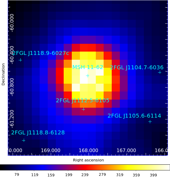
Fig . 1 TS map obtained fitting a source at each location of the map and computing the TS using gtlike. blue crosses represents the sources of the 2FGL catalog. MSH 11-62 is not included in the model.

Using pointlike, we searches for extension. First we refitted the sources in a ROI of 5° around MSH 11-62. We tested for extension assuming four shapes (point source, gaussian, disk and 2D gaussian) and computing the TS_ext.

As the source brigth, it is significant enough to allow us to test for extension using front events only (improving the PSF).

We tested for extension using the following enery-ranges (300 MeV-100 GeV, 1 GeV-100 GeV, 3 GeV-100 GeV, 5 GeV-100 GeV) and fitting the location and the extension. We found the greatest values of TS_ext using the 3 GeV-100 GeV energy range.

Tab. 1 Results of the test for extension in the ernergy range 3 GeV-100 GeV using all the events.

Tab. 2 Results of the test for extension in the ernergy range 3 GeV-100 GeV using front events only.

These results leads to the conclusion that the Fermi-LAT source 2FGL J1112.1-6040 is not significantly extended. Nevertheless, we found a 3 sigma evidence for extension of 0.1° (consistent with other wavelengths) and we need more data to conclude on the extension of MSH 11-62.

Spectral Analysis

As the spectrum seems to be well fitted  by either a Log Parabola or a Power Law+exp cut off we tried both assumptions.

Tab. 3. Parameters of the best fit obtained using gtlike and assuming a Log Parabola.

Tab. 4. Parameters of the best fit obtained using gtlike and assuming a power law + exp cut off.

We obtained the spectral points dividing the 100 MeV-100 GeV interval into 9 logarithmic-spaced bin. In each bin we fitted a powerlaw with a spectral index of 2.

Fig. 2. SED obained using gtlike. The statistic errors are represented in black and the systematic in blue. The blue line represent the best fit using a log parabola and the red one correspond to a power law +exp cutoff.The upperlimit are computed with a 3 sigma confidence level.

Systematics

Two main systematic uncertainties can affect the LAT flux estimation for a point source: uncertainties on the Galactic diffuse background and on the effective area. The dominant uncertainty at low energy comes from the Galactic diffuse emission, which we estimated by changing the normalization of the Galactic diffuse model artificially by 6% as done in Abdo et al. (2010). The second systematic is estimated by using modified IRFs whose effective areas bracket those of our nominal Instrument Response Function (IRF). These ”biased” IRFs are defined by envelopes above and below the nominal energy dependence of the effective area by linearly connecting differences of (10%, 5%, 20%) at log(E) of (2, 2.75, 4), respectively.

Cross checks :

1. Extension upper limit :

As asked during the Walk-through, we tried to derive an upper limit on the extension to estimate the systematics on this upper limit by changing the Galactic diffuse by +/- 6 %. The extension fit assumes a Gaussian shape and the upper limits are thus on the estimated sigma of the Gaussian. Here are the results for a 99%  bayesian upper limit :

Even though this upper limit is not stated in the paper anymore, this shows that the value 0.3° estimated previously was robust.

2. SED with front events only :

During the walkthrough, we have been suggested to verify that the SED (especially the low energy upper limits and points) are robust when using only front events. This is indeed the case as can be seen on the plot below (please note that the SED only includes statistical uncertainties):

3. Check for variability :

It has also been requested to verify whether the flux of the gamma-ray source associated with MSH 11-62 was really constant. This is indeed the case as can be seen below where the flux has been evaluated on a month time scale (upper limits are derived when the TS is lower than 9; the green point corresponds to a 2-week time scale of the point with highest flux which does not show any divergent behaviour):

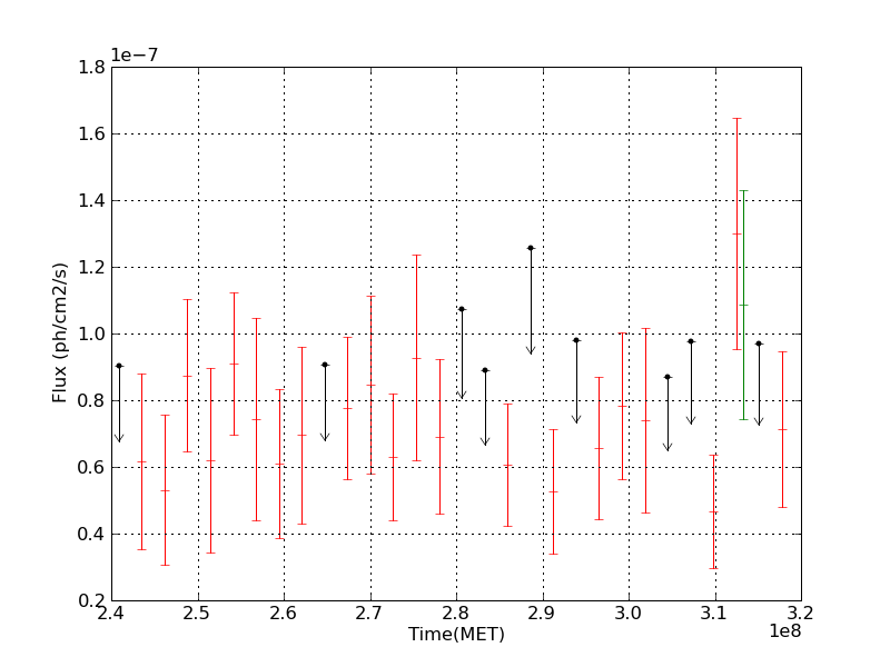
Using the same method as used in the 2FGL catalog, we can estimate TS_var = 13.83

• LAT Publication Board

draft v3, pub board page

draft v4 : 10/14/2011

Figures

Tables

Internal referee report 1 (Theresa Brand)

This paper seeks to identify the properties of the composite SNR MSH 11-62 and the processes and particles responsible for its multiwavelength emission.  The authors have obtained and analyzed high resolution data sets, including radio, X-ray, and gamma-ray data which greatly aid their mission. 
Where spatial resolution allows, they correlate emission processes with the particular regions of the composite SNR: pulsar, PWN, and SNR/shell. 
For the Fermi gamma-ray data, where spatial resolution does not allow such a precise correlation, they examine the hypotheses of emission from each region. 
Based on the multiwavelength spectrum and after ruling out the SNR and PWN scenarios under certain assumptions, including by comparison with similar known objects, the authors argue that, despite a lack of detected pulsations in any waveband, the 0.1-100 GeV gamma-ray emission most likely comes from the pulsar. 
It is a strong, generally well-written paper on important results and should thus be published pending resolution of the following general comments (below) and annotations (on the paper itself). 

Comments:

The authors are to be commended for gathering together and carefully analyzing the broad range of high-quailty data which allows them to draw substantial conclusions. Their generally transparent incorporation of the distance uncertainty into their work, including in stated luminosities, and inclusion of the hadronic component inherent in lepton-dominated SNR models is also worth noting.

General suggestions:

Pulsation search is standard for Fermi-LAT SNR analysis. Thus I would strongly encourage the authors to, minimally, obtain quantitative upper limits on the pulsed flux. The blind search done by Fermi-LAT members at Santa Cruz (et al) can be a good resource for this. Low-flux pulsars have also recently been detected by the Hanover group, which has further suggested that the young age indicated by this analysis merits expanding the search to higher-than-standard Fdot values. Such a search is already planned and should only take ~2 full(ly committed) days.  A pulsation detection would obvious greatly strengthen the pulsar-driven hypothesis. Quantitative upper limits would strengthen the statement that flux limits our ability to detect pulsations.
Likewise, it would be interesting to search for X-ray and radio pulsations, in particular if the expertise exists within or near the author team. 

A clearer discussion of how parameters were varied to fit the models to the (multiwavelength) data and, generally, quantifying statements, including the goodness of fit of the various models to the data would also greatly strengthen the paper. It is more difficult to exclude parameter space without having fully and demonstrably searched it. Likewise numerically comparing data to models yields clearer statements than, for instance, just visually observing a fit. This will help in particular in supporting the authors' preference for the pulsar scenario, which least-well fits the data with the smallest error bars, the radio and X-ray data.

In comparing the field and shell X-ray emission (section 3.4), it seems some assumptions are made, eg concerning the relative flux of the shell projected into the inside of the rim and any potential emission from within the shell itself. As this is a multiwavelength, analysis+theory paper, it could be particularly helpful to the broad range of readers to more explicitly state such assumptions. Moreover the authors might apply this even more extensively than they have already, throughout the rest of the paper. 

A side note: Unabsorbed vs deabsorbed X-ray data:
As I understand it, the X-ray spectral analysis tool xspec returns "unabsorbed" spectra. While this is common usage in X-ray spectrometry, it may lead to confusion in the wider audience interested in this paper as "un" implies not ever having been absorbed (eg), while "de" implies something which was absorbed and is no longer. The former suggests that we know the absorption perfectly, which is not true. The latter, while perhaps not the technical chemistry definition, was more readily understood as the process of removing absorption to estimate the intrinsic property in an open-ended poll of 3 non-X-ray-specialist astrophysicists.  
Given the conventional usage, using desorbed (or perhaps deabsorbed to more clearly differentiate from chemistry) is not requisite, but is suggested, as is considering the future use of the word.

other comments : MSH11-62_v3_commented_v1.pdf

Authors response to referee 1

I would like to thank Terri Brandt for her internal review of our
paper. Some of the many comments have uncovered typos that were
missed, and points for which some clarification would improve the
paper for non-experts. I've adopted those. Many of the points are,
in my opinion, style related, and for most of those I did not feel
that the suggested changes represented improvements, so I have opted
to maintain the original text or figures. For some of these, I
have explained why in my response below, where I have also explained
cases where the comments are simply incorrect.

A larger point of concern centers on a desire to approach the
modeling as a statistical fitting exercise. As I've described in
detail below, this is not the current state of the art in such
broadband PWN/SNR modeling, nor is it necessary to address the broad
issues we discuss here. I would note that Yosi Gelfand and I are
indeed working on Markov-Chain Monte Carlo modeling of such systems
in order to better assess how well the many free parameters can be
constrained in such exercises, but this is beyond the scope of our
MSH 11-62 analysis, and unnecessary for the model comparisons
presented here.General suggestions:

o Pulsation search is standard for Fermi-LAT SNR analysis. Thus I
would strongly encourage the authors to, minimally, obtain quantitative
upper limits on the pulsed flux. The blind search done by Fermi-LAT
members at Santa Cruz (et al) can be a good resource for this.
Low-flux pulsars have also recently been detected by the Hanover
group, which has further suggested that the young age indicated by
this analysis merits expanding the search to higher-than-standard
Fdot values. Such a search is already planned and should only take
~2 full(ly committed) days. A pulsation detection would obvious
greatly strengthen the pulsar-driven hypothesis. Quantitative upper
limits would strengthen the statement that flux limits our ability
to detect pulsations. Likewise, it would be interesting to search
for X-ray and radio pulsations, in particular if the expertise
exists within or near the author team.

I believe what you mean to say is that pulsation search is standard
for SNR analyses carried out by the Fermi-LAT team. That may be
true (I'm not sure), but it is surely not correct that all studies
of SNR emission using Fermi-LAT data include pulsation analysis,
nor do they need to. With regard to this particular study, there
have been no reports of detected pulsations from this source.
Informally, we have confirmed that a search was done with a null
result. Because of the low flux of the source, this result constrains
virtually nothing.

It is apparently true that there have been recent detections by the
Fermi-LAT team for lower flux sources. This is information that has
not appeared in the literature. We will not be referencing unpublished
work in this paper.

A pulsation detection would, of course, greatly strengthen our
conclusions. However, we have already discussed the prospects of
further searches with the Fermi-LAT pulsar team, and they agree
that if such pulsations were detected, they would want to write a
separate paper.

Searches for radio pulsations have been carried out by Fernando
Camilo, as stated explicitly in the paper. X-ray searches are
underway, but will be reported in a separate paper if detected.

o A clearer discussion of how parameters were varied to fit the models
to the (multiwavelength) data and, generally, quantifying statements,
including the goodness of fit of the various models to the data
would also greatly strengthen the paper. It is more difficult to
exclude parameter space without having fully and demonstrably
searched it. Likewise numerically comparing data to models yields
clearer statements than, for instance, just visually observing a
fit. This will help in particular in supporting the authors'
preference for the pulsar scenario, which least-well fits the data
with the smallest error bars, the radio and X-ray data.

I agree that clarification of the approach is needed. Text has been
added to explain that the modeling presented here does not represent
"fitting" of models to the data, nor does it represent an exhaustive
search of the complex parameter space. It focuses on three broad
model classes, and examines what primary impact measurable quantities
have on these models.

This modeling approach is the same as that used in virtually all
studies of the broadband emission of PWNe (see work by Fang et al.,
Bucciantini et al, Volpi et al., Fang et al., Zhang et al., and our
own group) and SNRs (see work by Ellison et al., Volk et al.,
Aharonian et al., Zirakashvili et al., Bykov et al., and others).
Concentrating on the goodness of fit here, and in other such studies,
is generally missing the point.

o In comparing the field and shell X-ray emission (section 3.4),
it seems some assumptions are made, eg concerning the relative flux
of the shell projected into the inside of the rim and any potential
emission from within the shell itself. As this is a multiwavelength,
analysis+theory paper, it could be particularly helpful to the broad
range of readers to more explicitly state such assumptions. Moreover
the authors might apply this even more extensively than they have
already, throughout the rest of the paper.

I'm not at all sure what "comparing the field and shell X-ray
emission" means, but this presumably refers to the method used for
the density estimate. This calculation, described explicitly as
"Based on the volume emission measure... and assuming a thin-shell
morphology for the SNR, with a shell thickness of R/12 corresponding
to a shock compression ratio of 4", is the most standard way there
is of estimating the density from an SNR using the X-ray spectrum.
It is used in countless papers. The volume of a thin shell is given
by 4*pi*R2*l, where l is the shell thickness. The volume emission
measure is obtained from the X-ray fit and is proportional to n2*V.

o A side note: Unabsorbed vs deabsorbed X-ray data: As I understand
it, the X-ray spectral analysis tool xspec returns "unabsorbed"
spectra. While this is common usage in X-ray spectrometry, it may
lead to confusion in the wider audience interested in this paper
as "un" implies not ever having been absorbed (eg
<http://www.wordnik.com/words/unabsorbed>), while "de" implies
something which was absorbed and is no longer. The former suggests
that we know the absorption perfectly, which is not true. The latter,
while perhaps not the technical chemistry definition
<http://www.wordnik.com/words/desorb>, was more readily understood
as the process of removing absorption to estimate the intrinsic
property in an open-ended poll of 3 non-X-ray-specialist astrophysicists.
Given the conventional usage, using desorbed (or perhaps deabsorbed
to more clearly differentiate from chemistry) is not requisite, but
is suggested, as is considering the future use of the word."""

I'm afraid that this description is exactly backwards. In modeling
X-ray spectra, one does indeed start with a model that is free of
any absorption. One then applies the absorption on top of this,
multiplies by the effective area curve, and convolves with the
instrument spectral redistribution matrix. This has nothing to do
with xspec; all X-ray modeling is done the same way. The model thus
starts with an unabsorbed flux, and this is converted to a modeled
observed flux by applying absorption (as well as detector
characteristics), which is then compared with the data. The reported
flux is that of the best-fit model. The unabsorbed flux is just the
starting flux of the model. This is the terminology that has been
in use for decades, and in many thousands of papers, and it is an
apt description.

Specific items from marked-up pdf file:

o un-italicize the '2' -

No. This is the correct nomenclature. See, for example, the reference
to the original "MSH" paper that we cite in the Introduction.

o improving our understanding

Fixed.

o reference?

Same reference. I combined this into a single sentence to remove any
confusion.

o Is there further motivation for 5kpc than >3.5kpc and within the galaxy?

No.

o It would be helpful to have consistent coordinate systems on all
wavelenghts' sky maps (eg Fig 2, 3, 5, 7, ...). It would also be
useful to have intensity (color) scales labeled (eg Fig 1,
... ).

This has already been done for several of the figures, and these
are included in the revised version. Figures 2 and 5 require a bit
of fussing to apply coordinate grids, but I will add those.

As for Figure 1, the levels are already specified for the contours.

o southWestern?

Indeed. Fixed.

o It would be helpful to include a note on the circled, red sources.
Presumably these are the excluded point sources associated with Tr
18?

Correct. I've added a note to the caption.

o It would be nice to clarify how this correlates with not having
FoV in the NE. Perhaps something like: "the emission appears to lie
entirely within the detector field of view and thus does not extend
as far to the NE as the radio bar" ? This might also be clearer
with axes on the Xray image.

Axes have been added to Figure 3, and will be added to Figure 5.
It should already be evident from Figure 3 that the X-ray emission
from the PWN does not fall off the edge of the chip, since the PWN
and the chip edge are readily discernible in the image. Similarly,
it should be evident from Figure 5 that the PWN emission in the XMM
image does not extend to the northeastern boundary of the radio
PWN.

o Does the limb-brightening in the east also align in the X-ray and
radio?

Roughly. Please see Figure 5.

o Excluding CXOU J111148.6-603926 ?

Correct. I've clarified in that sentence.

o From Table 1, Gamma ~1.8.

Fixed.

o Would it be possible to show the background region on one of the figures?

No. Too cluttered.

o Please use comparable numbers, eg Chandra luminosity/XMM luminosity rather
than Chandra flux/XMM luminosity.

I think you're missing the point being made here. The text says
that fits from Chandra and XMM are virtually identical (which implies
the fluxes are the same). The luminosity is then provided for
comparison with both physical processes and with previous published
results. It is the same for both Chandra and XMM results.

o Any thoughts on why Kargaltsev & Pavlov got such a high value?

Nope. I have no idea how they got this. They don't give any detailed
information in their paper.

o It would be nice to have the XMM pn PWN observation here too.

There is already a sentence stating that the results are the same
as those from the Chandra spectrum. There seems little point to
adding three more lines to a table to reiterate this.

o Such steepening

Fixed. (Hmm... beginning to look like I didn't spell-check after my last
round of edits...)

o Are there PWNe which do not follow this trend?

I'm not aware of any that unambiguously do not follow the trend,
but there are certainly plenty for which the data aren't good enough
to demonstrate that they do.

o Would it be possible to show the compact source integration region
on a figure (eg 3)?

It is much smaller than the burned-in image of the compact source
in that image (which has been smoothed and stretched to show the
PWN). I'm a bit confused about why one would need to see that when
the source itself is perfectly clear, and the radius of the extraction
region is stated.

o What are the col density and index if the col density is free?

N_H = (9.3 +3.5 -2.3) x 10^21Gamma = 1.4 +0.2 -0.3

o Would it be possible to show the background regions in the figure (5)?

Yes, but at the expense of shrinking the actual emission region.

o How good is the fit? How much better is it than a simpler model?

Chi-squared is 768.5 for 612 degrees of freedom.

A single temperature model gives chi-squared of 909.4 for 614 degrees
of freedom.

o How much better is the fit with a thermal component rather than a power
law?

Only marginally better. Chi-squared is 774.6 for 612 degrees of
freedom with the power law. I've changed the wording to better
describe the difference in the fits.

o What are the results of the blind pulsation search for this object?

We did not carry out a Fermi timing analysis. However, members of
the Fermi-LAT team have, and did not detect anything of significance.

o It can be helpful to include the actual UTC (or MET) start and stop times.

This is a bit superfluous. The data span more than 2.5 years, and we have
specified it to the day. Specifying UTC start/end times will refine that
interval by no more than 0.1%...

o No need for quotes: it's called Pass 7v6

Changed to Pass 7 version 6

o was modeled (maintain the same tense)

Fixed.

o For what energy range and position is this TS? It might be helpful
to tell readers you'll discuss extension and localization shortly.

Text has been modified to clarify this.

o Are the pulsars detected by the LAT? If so, what is their effect
on the LAT detection? particularly at lower energies? When you
"ignore" their contribution, what does this mean for the likelihood
analysis?

No, they are not.

Concerning PSRJ 1112-6103 there is a 2FGL source (2FGL 1112.5-6105)
but no pulsation was detected. The influence of this pulsar should
be a systematic at low energy but Josh did an SED without relocalizing
PSRJ 1112-6103. Romain did relocalize it and the results are the
same on the model. He thinks these pulsars are part of the low
energy systematics, but not the biggest.

By "ignore their contribution" we mean that in subsequent analysis
regarding the physical properties of MSH 11-62, we attribute all
of the gamma-ray emission to this source.

o What is the TS or significance of the PL with EC fit? versus a
plain PL?

It represents an improvement at the 6.8 sigma level. This has been
added to the text.

o These are the main systematics for point sources in the galactic
plane.

It would seem that most people realize that uncertainties in the
Galactic diffuse background aren't the dominant issue at high
latitude, but we've added "in the Galactic plane" to be sure.

o We usually use the term bracketing IRFs, rather than biased.

Fixed.

o It might keep things clearer if you used the same color for the
(Fermi) data points and errors for all the plots.

We are confident that the reader will realize that only one gamma-ray
data set is being introduced here.

o What does the "red error bars including the systematics" mean?
as well as the statistical? This implies the two types are added...
in quadrature? Or, as I suspect, do the red error bars just show
the systematic errors?

Black error bars correspond to statistical errors, while red error
bars correspond to both the statistical and systematic errors.

o What shape was used for the extended hypothesis? (Gaussian,
disk,...)

Added "We fitted the position of the source assuming iteratively a
point source and a Gaussian shape for which we fitted the extension.

o Did you simultaneously fit the position and extension?

Yes.

o It might be nice to include an estimate of when Fermi might
accumulate sufficient statistics (given the current tools/PSF/etc).

With no knowledge of the actual extent, nor or its morphology, this
would be a purely speculative exercise.

o Either italicize TS or don't.

Fixed.

o It would be helpful to have the sections referenced, rather than
just "text". (Figures 8 & 9)

Fixed.

o Since the observed radius is a function of the distance, these
values should also reflect that, as nicely done for the luminosities.

This is true, but here we have referred explicitly to numerical
values assumed for the model. In that case, there is a well-defined
radius.

o It is not necessary but could be helpful to non-expert readers
to redefine RS here.

Converted to "reverse shock"

o It would be helpful to more explicitly say how a RS-PWN interaction
would a give distorted morphology.

The rest of the sentence does explain this more explicitly: "which
appears to indicate that the RS has propagated most rapidly along
the NW/SE direction"

o As this is an important figure, it could be worth making it bigger
so the features are easier to see.

The actual size is indeed large. It all depends on how ApJ prints
it. However, I'm not sure what could be made easier to see except
for the bow-tie, which I have now plotted in black.

o Please make the radio data an actual bowtie.

It is an actual bowtie. It's just that the uncertainties are small
for a plot that covers this much frequency and flux space.

o It would be useful to define the lines and points in the caption.

Fixed.

o Quantitatively how good is the fit? How did you search the parameter
space to determine the reported values? How do the results change
with distance?

As described above, goodness-of-fit statistics were not used here.
The parameter space was explored by systematically varying the
dominant parameters by hand first, then fine-tuning other parameters
by hand. The distance behavior can be inferred from the discussion,
where we discuss results for smaller distances.

Text has been added to more fully describe this process.

o Please indicate what is used to determine the flux/make the bowtie
in Figure 10, eg, "and used a spectral index range of alpha =
0.4-0.7, typical of radio emission from shell-type SNRs, to limit
the flux to the bowtie in Figure 10."

I don't understand. This is exactly what the paper says: "Here we
have used the measured 1.4 GHz flux from the shell, and assumed a
spectral index range of "gamma_r = 0.4 - 0.7 typical of radio
emission from shell-type SNRs." The only thing missing is the word
"bowtie"...

o It could be helpful, as was done for Table 1, to indicate in the
table which parameters have been fixed and also to include k_e-p.

Added k_ep. Indicated that this, and distance, are fixed.

o Have you tried fitting the hadronic scenario with a preshock
density closer to the one inferred from Xrays? Showing quantitatively
that it poorly reproduces the data (or conversely, using the data
to rule out such low preshock densities) would strengthen the
conclusion: not hadronic-dominated.

No, because the result such a model would yield is already obvious.
The flux scales with the ambient density, so it will be a factor
of nearly 200 fainter if we use the value derived from the X-ray
emission. It is thus not a model of interest.

o Masers are fairly finicky creatures, requiring pretty specific
conditions and viewing angles, so not seeing one doesn't necessarily
imply no dense material. Have you checked gas maps of the region
for other tracers of dense material? Though the uncertain SNR
distance measure will not permit perfect association, one can
probably rule out at least some of the gas based on the velocity-distance.

Yes, we've already modified the text here to make even clearer the
fact that lack of maser emission doesn't rule out ambient material.

We have not carried out searches through data cubes of molecular cloud
emission. Without detailed line profiles (and often even with them), such
techniques are rarely productive in establishing connections between
SNRs and dense clouds.

o How does the model change if you allow the ambient density to
vary (eg increase)?

The results are the same until the density gets to the point where
the pion component starts to be comparable to the IC component. At
that point the problem with the large electron energy goes away and
the problem with the very high ambient density is in place. There
isn't a solution (for 5 kpc) in which the electron energy is modest
and the ambient density is anywhere close to the X-ray value.

o How much do the other photon fields in the region contribute?

Very little to the Fermi band.

o Does the model require the super-exponential cutoff or does the
best fit of the model to the data require it? What is the quantitative
improvement in the model fit when including the super-exp cutoff?

I'm not sure I understand this question. Are you asking if we only
have a super-exponential cutoff model, for which we can't set b =
1 (in equation 1)? If so, then no.

As mentioned above, the "fits" here are done "chi-by-eye." What
this means is that if you don't use b > 1 in the leptonic case, you
simply can't get the curve to go through the points.

o shows the associated electron distribution?, which is modeled
as...

Fixed.

o Making the distance dependence more transparent in the previous
paragraph's leptonic scenario discussion would strengthen this one.

I'm not sure how to make it any more transparent. We considered the
case of a 5 kpc distance, reported the problems, then explained
that they get better, but still don't go away, even if we move to
the smallest reasonable distance (and we present the numerical
values for this distance). That seems to provide adequate information
for the reader to understand the point here.

o Please be explicit about the caveats to this statement, eg the
assumed density.

As noted above, this doesn't depend on the density. For the leptons
to dominate, there has to be a huge amount of energy in the electron
spectrum. If the density goes way up, the electrons no longer
dominate, and we're no longer discussing a leptonic scenario.

o Thanks for showing which variables were fixed. It might be easier
to see at a glance if the word fixed were associated with the
variable name, rather than its value.

Fixed.

o Were the IR field parameter values within their respective error
limits?

This is answered in the next sentence of the paper: "The final
values listed in Table 3 are within reasonable expectations for
this region of the Galaxy (see Strong et al. 2000)."

o Worth noting: We found that it was not possible to ... under these
assumptions.

Added.

o Quantitatively, how good is the fit? compared to the power law
or broken power law particle spectrum models?

See other comments on goodness of fit questions.

o Please use section number here, rather than just "above".

Changed to "as discussed in Section 5.1"

o Please define gamma.

We have added "a Lorentz factor"

o Using the XMM luminosity of 1.1x1034 ergs/s and the Edot in this
paragraph, I get Lx/Edot ~1.3x10-5 d52. ~10-6 is consistent
with Lx/Edot_0, but presumably Lx and Edot should be of the same
epoch, as suggested by the variable names. Please clarify.

Yes, this should say 10^(-5). It has been fixed.

o Great that you checked to the limits of the distance uncertainty.
Does the model become more feasible if you change the breaking
index? This is particularly crucial as this affects the spin-down
power and thus the inferred (extremely low) conversion, upon which
the main rejection of the PWN hypothesis is based. How large is the
effect of changing other previously fixed parameters to other
reasonable values?

Reducing the braking index (the only realistic scenario) requires
an increase in the initial spin-down power. Thus, it makes the
problem worse.

o The X-ray PWN emission?

The X-ray and radio emission. I've clarified in the text.

o It would be nice to explicitly show how the distance contributes
to the stated ambient density value.

This calculation holds for a distance of 5 kpc. We've added that
statement to the text.

o How do you derive these values? Quantitatively how good is the
fit to the data? For instance from the previous paragraph, I had
expected Lx/Edot fixed at 10-3.

The values come from the model that is explained earlier in the
paper. The model uses Edot_0 as an input parameter. It evolves the
PWN and SNR with time. Using the value of n_0 measured in X-rays,
the observed SNR radius is reached in 700 years. The evolved PWN
magnetic field is then that given in the paper. Lx/Edot isn't known,
so this can't be used as a model input.

I've modified the text here a bit to help clarify this.

o Please comment on the fact that there appears to be the greatest
discrepancy between the X-ray and radio data and the model in the
favored, pulsar-powered scenario.

There isn't much to comment on. The model parameters have not been
adjusted with infinite flexibility to obtain a fit. It is a mistake
to keep thinking of the results in a "best fit" sense. That's completely
the wrong thing to concentrate on in this paper.

o The paper makes something of a point of the asymmetric radio- and
X-ray -detected PWN morphologies. It might be interesting to quantify
this and compare it to the asymmetry one might expect from models.

This requires 2-D (or 3-D) hydrodynamical simulations, beyond the
scope of this paper.

o Mexico

Fixed

o Discussion in section 5.3 seemed to suggest that the PWN scenario
was inconsistent with the X-ray flux relative to spin-down power
given a fit to the gamma-ray flux.

Yes, this is correct. I'm not sure what the point is here. Section
5.3 shows that if the gamma-ray emission arises from the PWN, then
the Edot required for the pulsar is very high, leading one to expect
a high gamma-ray flux from the pulsar itself (which, of course,
then means the gamma-ray emission doesn't arise from the PWN,
contradicting the hypothesis). The inferred Edot value is also very
high for the observed X-ray emission. That's just what the summary
statement says here.

o extension

Fixed

internal referee report 2 (name)

Authors response to referee 2

Journal referee report

Referee Report  

This paper combines observations of the composite supernova remnant MSH
11-62, taken in four different spectral ranges, that have been already
published only in part. The most recent data are those taken with the Fermi
LAT, and in fact the various scenarios discussed all start from different
hypotheses on the origin of the emission detected in the GeV range.

The idea is interesting. However, the analysis of the parameters for the
various models does not seem to be exhaustive. Therefore, I believe the paper
will eventually deserve publication, but I recommend a more detailed
discussion of some points plus a series of clarifications, along the lines
listed below.

The authors point out something like the following: "In these model
investigations, we have varied input parameters to investigate the broad
effects they have on the broadband spectrum, and have then fine-tuned
parameters to provide reasonable agreement with the data. The resulting
models are not statistical fits to the observed emission, and were not
optimized by a likelihood analysis over the large parameter space." Even
without requiring a fully formal approach, it is not clear enough whether the
parameter space has been explored enough to confidently exclude the existence
of other valid solutions. In other words, it is not clear that Tables 2 and 3
give the "best" parameters for all proposed models. But the number of
parameters is larger than the number of the observational constraints. It
would have been nice if, for instance, among all these parameters the authors
singled out  the ones (only a few, hopefully) which are the leading, most
relevant ones.

Just as an example, in the last case presented (that in which the gamma-rays
come from the pulsar) the pulsar wind nebula (PWN) model is constrained just
by the radio and the X-ray data. Among the derived parameters there is a PWN
field of about 13 muG, namely a factor 5 lower than the minimum energy
magnetic field. On the other hand, a previous work (Harrus, Hughes & Slane
1998) was able to reproduce both the radio and X-ray data available at that
time using a minimum energy magnetic field. Even though data and models are
now more accurate, I am wondering what is the reason of such a large
discrepancy with respect to the older model. Maybe the Harrus et al. model
was wrong? Or the best-fit (or sort of) model is not unique? In other terms,
I may understand the requirement of a very low magnetic field, if the same
particles are used to explain both the radio (synchrotron) and the (IC)
gamma-rays; but I am missing why it must be so, also when a different origin
for the gamma-ra
ys is
invoked. The authors should provide a more detailed discussion of this point.

By the way, the derived ratio between the magnetic field energy and that of
relativistic electrons in the PWN is an important physical parameter. While
the minimum-energy case prescribes an almost perfect equipartition (3/4), in
the above model (with B~13 muG) the ratio is much lower, about 1/370 (i.e.
5^(-7/2)*3/4). Even lower values are obtained for the other models, because
even lower magnetic field strengths are derived, and in addition because in
the presence of a prominent Maxwellian component the energetics of radio
emitting electrons are no longer representative of the total energy of the
electron component. For instance, for the case presented in Fig. 11 I have
roughly estimated a ratio of about 10^(-6). Even though there is no a priori
reason for equipartition to be always closely matched, a deviation of 6
orders of magnitude is so large that needs to be justified.

What is taken as the PWN size, in the illustrative model for the evolution
(Page 15, Fig.9)? Its value along the NE-SW direction? Or that along the
SE-NW direction? Or a combination of the two? By a rough estimate based on
Fig.1 and Fig. 9, I have derived a PWN diameter of about 8 arcmin, namely
even larger than the PWN seen along the NE-SW  direction. What is its right
value? Also, I am puzzled by the fact that, from the model as well as from
the estimated PWN magnetic strength, it seems like the interaction with the
SNR shell has just started, while the PWN flat shape seems to indicate that
the reverse shock has already squeezed the PWN, at least along the SE-NW
direction. This issue is mentioned a few times in the paper, but is not
discussed. For instance, it is not quite clear the meaning of the sentence
"This appears consistent with the X-ray and radio morphology" (Page 18, which
by the way seems to be contradicted by the next sentence).

OTHER POINTS:

Page 10. About the spectral stepping in 3C 58, there is a reference (Bocchino
et al. 2001) earlier than that cited (Slane et al. 2004).

Page 11. I do think the information Delta chi^2=6.1 has any meaning, if the
number of degrees of freedom is not given.

Page 13. Some more words on the "Test statistic" (does it correspond to the
"likelihood ratio test" in Mattox et al. 1996?) should be added, at least to
define it, to give the formula for translating it into a sigma value, and to
specify how the significance levels translate into position uncertainty of
the detected source.

Page 14. About the 0.1 degree size determination, can one also estimate its
(1-sigma) uncertainty? To which confidence level one can exclude that a minor
contribution from another nearby pulsar contributes to the quoted (marginal)
extension?

Page 14. A reference should be given to the routine POINTLIKE.

About the leptonic SNR case, it is shown in Fig. 8 and 10, and mentioned in
the Conclusions, but virtually nothing is said in the section in which it
should have been discussed (Page 17).

Page 19. de Jager, Slane & LaMassa 2008 suggest the coexistence of two
different power-law components, but do not mention any Maxwellian component.

Table 1
What is the difference between the "fixed" value NH in model #4, with respect
to model #2 and #3? It is not quite clear from the table.

Typos:
Page 12. "instrument instrument"- Page 13. "to to"

Authors response to the referee

Response to Referee Report  

We thank the referee for the detailed comments on this manuscript.
We have addressed these in the revised version, and below we provide
a detailed reply to each comment.

First, and foremost, we must apologize for two rather egregious
mistakes in the original manuscript. First, in the process of
converting the text into the final ApJ format, three full paragraphs
from Section 5.2 were inadvertently deleted. This removed the entire
discussion about the lepton-dominated scenario, which the referee
notes. This clearly made the entire argument quite convoluted.
Second, the axis for the top panel in Figure 11 was mislabeled.
While the label states that Log (E dN/dE) was plotted, in reality
the plot showed Log (1/E)(dN/dE).  This was not intentional. The
bottom panel plots E^2 dN/dE for the photons. For the upper panel,
the plotting command from the bottom panel was replicated, and then
multiplied by 1/E to yield E dN/dE for the electrons. However, what
had actually been read in for the electron spectrum was dN/dE, not
E^2 dN/dE. Dividing by E thus provided 1/E dN/dE, not E dN/dE as
intended.  This lead to the (quite correct, based on the plot)
concern by the referee that the particle and magnetic energy densities
were wildly different from the minimum energy condition. We have
fixed the plot, and discuss the energetics below. Again, apologies...

We have provided a "red-lined" version of the revised manuscript
in which the modifications to the text and tables have all been
indicated in red.

> This paper combines observations of the composite supernova remnant
> MSH 11-62, taken in four different spectral ranges, that have been
> already published only in part. The most recent data are those taken
> with the Fermi LAT, and in fact the various scenarios discussed all
> start from different hypotheses on the origin of the emission
> detected in the GeV range.

It is a small point, perhaps, but we would suggest that this
description underplays the analysis presented here rather considerably.
Preliminary results from the radio observations were presented by
our group in a couple of conference proceedings, one of which also
mentioned the discovery of a point source in the Chandra data, and
an image (and an incorrect luminosity estimate) of only the center-most
region of the Chandra observations was presented by another group
in another conference proceedings.  The gamma-ray source is listed
in the first Fermi LAT catalog, as a potentially confused source.
The ATCA, Chandra, and XMM data have not been presented in any
refereed publication, nor have the Fermi LAT image or spectrum.  No
quantitative analysis of the radio or X-ray data have been presented
in any form.  In addition, while it is indeed correct that the
various scenarios described in the discussion center on the origin
of the GeV emission, this is because the gamma-ray data, by themselves,
are the least constraining. It is only by combining the results
from the other observations that we can address physical scenarios
for the source of the gamma-ray emission. The focus of the paper
is on the multiwavelength properties of MSH 11-62, not just the
gamma-ray emission.

> The idea is interesting. However, the analysis of the parameters
> for the various models does not seem to be exhaustive. Therefore,
> I believe the paper will eventually deserve publication, but I
> recommend a more detailed discussion of some points plus a series
> of clarifications, along the lines listed below.
>
> The authors point out something like the following: "In these model
> investigations, we have varied input parameters to investigate the
> broad effects they have on the broadband spectrum, and have then
> fine-tuned parameters to provide reasonable agreement with the data.
> The resulting models are not statistical fits to the observed
> emission, and were not optimized by a likelihood analysis over the
> large parameter space." Even without requiring a fully formal
> approach, it is not clear enough whether the parameter space has
> been explored enough to confidently exclude the existence of other
> valid solutions. In other words, it is not clear that Tables 2 and
> 3 give the "best" parameters for all proposed models. But the number
> of parameters is larger than the number of the observational
> constraints. It would have been nice if, for instance, among all
> these parameters the authors singled out  the ones (only a few,
> hopefully) which are the leading, most relevant ones.

This is a very fair and reasonable concern, and one that we actually
have tried to address, but clearly need to refine. We note that the
additional text (which was inadvertently deleted) on the leptonic
scenario for the case in which the SNR dominates the gamma-ray
emission (Section 5.2) helps to clarify this a bit, because we
describe how we arrived at some of the numerical values in Table
2.

We have modified the discussion in Sections 5.3 and 5.4 to better
clarify how the modeling was carried out, and which parameters let
to sufficiently small changes to allow us to set them to fixed
values.  One such parameter is the ambient density, and to simplify
matters we have fixed this to be the same in the models for which
the PWN and the pulsar dominate the gamma-ray emission.  Small
parameter changes are indicated in red in Table 3, where we have
also (hopefully) done a better job of indicating which parameters
were set to initial values and then fixed when modeling the emission.
In addition, in Figure 11 we now show models for different values
of the ambient density in order to provide some indication of the
sensitivity to changes in parameter values.  We have also corrected
a typo for the break energy.

We have added a comment about the overall fidelity of the model
parameters listed in Table 3, noting that variations in the distance,
for example, can produce significant changes, but that the primary
conclusions pertaining to the high spin-down energy and the particle
dominance of the energy density are robust.

In addition, while we discussed results for both the nominal 5 kpc
distance as well as for a smaller distance in Section 5.4, we
originally listed the models values for the smaller distance in
Table 3. To avoid confusion, we have revised this to list model
parameters for the same 5 kpc distance that was used for Section
5.3. The results obtained when considering a smaller distance are
still discussed in the text.

> Just as an example, in the last case presented (that in which the
> gamma-rays come from the pulsar) the pulsar wind nebula (PWN) model
> is constrained just by the radio and the X-ray data. Among the
> derived parameters there is a PWN field of about 13 uG, namely a
> factor 5 lower than the minimum energy magnetic field. On the other
> hand, a previous work (Harrus, Hughes & Slane 1998) was able to
> reproduce both the radio and X-ray data available at that time using
> a minimum energy magnetic field. Even though data and models are
> now more accurate, I am wondering what is the reason of such a large
> discrepancy with respect to the older model. Maybe the Harrus et
> al. model was wrong? Or the best-fit (or sort of) model is not
> unique?

Harrus, Hughes, & Slane (1998) presented three different estimates
of the magnetic field. The first was based on the radio synchrotron
spectrum, the estimated size of the nebula, and minimum energy
assumptions.  The radio flux, shown in Figure 5 of that paper, was
based on early radio measurements and correspond to the entire
source. The results from our more recent observations provide a
lower flux for the PWN region. This reduces their value by about
30%. In addition, we use the radius from our dynamical model, which
is larger than that adopted by Harrus et al. by about 35%; this
radius reduces their value by about another 30%, to a final value
of about 36 uG for a distance of 5 kpc. In any case, this is not a
model calculation of the magnetic field; it is simply a calculation
of the magnetic field under minimum energy assumptions, which may
or may not hold. Our current model does indeed indicate a large
deviation from equipartition.  Similar results have been reported
for W44 (Bucciantini et al. 2011), G0.9+0.1, and G338.3-0.0 (Fang
& Zhang 2011).  We do not feel that the value implied by our results
is unrealistic.

The other estimates provided by Harrus et al. are highly uncertain.
The second is based on an inferred spectral break between the radio
and X-ray band (again using the full radio flux, rather than only
the fraction associated with the PWN), but observations of other
PWNe (e.g., 3C 58 and G21.5-0.9) show that the broadband SED of
PWNe can be more complicated than a simple double power law
extrapolation. The third magnetic field estimate assumes pressure
equilibrium between the PWN and the SNR interior. The latter was
difficult to measure because the thermal X-ray spectrum was poor,
but the results from such a calculation are highly uncertain in any
case, for several reasons: the pressure depends on the state of
temperature equilibration between electrons and ions; the thermal
X-ray emission, which shows no strong evidence for ejecta, may not
reflect the conditions at the reverse shock; and the degree of
pressure equilibration between the  PWN and the reverse shock depends
on the evolutionary state.

We have added further discussion to summarize the above.

> In other terms, I may understand the requirement of a very
> low magnetic field, if the same particles are used to explain both
> the radio (synchrotron) and the (IC) gamma-rays; but I am missing
> why it must be so, also when a different origin for the gamma-rays
> is invoked. The authors should provide a more detailed discussion
> of this point.

The constraint that dominates the magnetic field value is provided
by the X-ray spectrum of the PWN. While it is possible to construct
scenarios in which the magnetic field is stronger, by increasing
the fraction of the injected energy that is in the form of magnetic
flux, this results in larger synchrotron losses, leading to a cutoff
below the X-ray band. The resulting spectral index in the X-ray
band is much steeper than observed. We have added text to clarify
this point.

> By the way, the derived ratio between the magnetic field energy and
> that of relativistic electrons in the PWN is an important physical
> parameter. While the minimum-energy case prescribes an almost perfect
> equipartition (3/4), in the above model (with B~13 uG) the ratio
> is much lower, about 1/370 (i.e.  5^(-7/2)*3/4).

As noted above, the deviation isn't quite this large. But indeed
our results imply a particle-dominated nebula, similar to results
found for a number of other evolved PWNe.

> Even lower values
> are obtained for the other models, because even lower magnetic field
> strengths are derived, and in addition because in the presence of
> a prominent Maxwellian component the energetics of radio emitting
> electrons are no longer representative of the total energy of the
> electron component. For instance, for the case presented in Fig.
> 11 I have roughly estimated a ratio of about 10^(-6). Even though
> there is no a priori reason for equipartition to be always closely
> matched, a deviation of 6 orders of magnitude is so large that needs
> to be justified.

Indeed this would be a pretty worrisome result! However, this just
reflects the plotting error in Figure 11. The actual ratio of
magnetic energy density to particle energy density for the particular
case with the Maxwellian distribution is about 4e-3. (Here we have
integrated the electron spectrum, not inferred the particle energy
density by modeling the radio emission assuming a power law particle
population.) Thus, with the corrected figure we believe this issue
has been addressed.

> What is taken as the PWN size, in the illustrative model for the
> evolution (Page 15, Fig.9)? Its value along the NE-SW direction?
> Or that along the SE-NW direction? Or a combination of the two? By
> a rough estimate based on Fig.1 and Fig. 9, I have derived a PWN
> diameter of about 8 arcmin, namely even larger than the PWN seen
> along the NE-SW  direction. What is its right value?

The value used here is that from the dynamical model (that is, the
field is calculated continuously as the system evolves), which is
a radius of about 5 pc for the age indicated in Table 3. This
corresponds to an angular diameter of 6.9 arcmin at a distance of
5 kpc, which is in good agreement with the observed long axis of
the PWN. We have now stated the value explicitly in the text.

> Also, I am
> puzzled by the fact that, from the model as well as from the estimated
> PWN magnetic strength, it seems like the interaction with the SNR
> shell has just started, while the PWN flat shape seems to indicate
> that the reverse shock has already squeezed the PWN, at least along
> the SE-NW direction. This issue is mentioned a few times in the
> paper, but is not discussed. For instance, it is not quite clear
> the meaning of the sentence "This appears consistent with the X-ray
> and radio morphology" (Page 18, which by the way seems to be
> contradicted by the next sentence).

Yes, we totally agree with this statement, and it is really exactly
what we were trying to say with the above sentence - namely: 1) the
fact that the model indicates that the RS is interacting with the
PWN is consistent with the fact that the PWN morphology seems to
indicate it has been crushed; but 2) the crushing actually seems a
bit larger than we expect from the model. That is, we have some
level of qualitative agreement, but not strict quantitative agreement.
We've reworded this to remove what apparently seemed like a
contradiction in the same sentence. With regard to the flat shape
of the PWN, we suspect that this is telling us that the RS interaction
has occurred asymmetrically, which is something that our spherical
model is not capable of simulating. We've added a sentence to express
this.

> OTHER POINTS:
>
> Page 10. About the spectral stepping in 3C 58, there is a reference
> (Bocchino et al. 2001) earlier than that cited (Slane et al. 2004).

Ah, that's right! Bad oversight. This has been added.

> Page 11. I do think the information Delta chi^2=6.1 has any meaning,
> if the number of degrees of freedom is not given.

We've added the number of degrees of freedom now.

> Page 13. Some more words on the "Test statistic" (does it correspond
> to the "likelihood ratio test" in Mattox et al. 1996?) should be
> added, at least to define it, to give the formula for translating
> it into a sigma value, and to specify how the significance levels
> translate into position uncertainty of the detected source.

Sorry, this has become jargon in the gamma-ray community. We've
modified this sentence to provide a better description of this.
The significance levels translate more into an indication of possible
extent (or, in this case, of an unresolved source).  We have also
clarified this in the text.

> Page 14. About the 0.1 degree size determination, can one also
> estimate its (1-sigma) uncertainty? To which confidence level one
> can exclude that a minor contribution from another nearby pulsar
> contributes to the quoted (marginal) extension?

We are not claiming that the emission is extended. There is no
significant evidence for this. We have reworded the text pertaining
to extended emission to make this more clear.

> Page 14. A reference should be given to the routine POINTLIKE.

This has been added.
 
> About the leptonic SNR case, it is shown in Fig. 8 and 10, and
> mentioned in the Conclusions, but virtually nothing is said in the
> section in which it should have been discussed (Page 17).

Yes, this text was inadvertently deleted. It has been restored.

> Page 19. de Jager, Slane & LaMassa 2008 suggest the coexistence of
> two different power-law components, but do not mention any Maxwellian
> component.

The text doesn't actually say that the above reference identifies
a Maxwellian component; it states that it identifies a distinct low
energy component. We've modified the text to note that it was modeled
with a power law.

> Table 1 What is the difference between the "fixed" value NH in model
> #4, with respect to model #2 and #3? It is not quite clear from the
> table.

Sorry, the value for model #4 should also read 6.7e21, and have a
pointer to the note that indicates it is fixed at the best-fit value
for the PWN. We used the same N_H value for models 2, 3, and 4.
We've fixed the table.

> Typos: Page 12. "instrument instrument"- Page 13. "to to"

Fixed.

• SCIENCE GROUP PAGES
• LAT Speaker Bureau
• Templates for Presentations
• OTHER LINKS

  Error rendering macro 'deck'

  java.lang.NullPointerException

  General suggestions: