Presentation FERMI _HBL presentation.pdf
HBL_answers_agncoordinators.docx
Internal reviewer comments on the April, 2019, ApJ version
Changes made April, 2019, due to suggestions from Vaidehi:
Updated wording as suggested
Dropped TSvar, because that variability analysis was not used in the paper.
Combined and consolidated tables.
Response to the ApJ Review:
We extend our thanks to the referee for a careful reading and helpful suggestions. Responses to the recommendations are given below. Changes in the text appear in bold font.
- The authors should explain why they decided to perform the extrapolation of the SED for high-confidence HSPs sources
only, i.e. with L_HSP>=0.89. Based on the estimated purity of their classification based on the validation of their machine
learning method reported at the end of Section 2, a lower L_HSPs>0.8 threshold will still produce a 75% efficiency that
would probably yield a quite large number of HSPs detectable by IACTs under the same assumptions used for the
high-confidences ones. Is this study a proof-of-concept that will be extended to the other (slightly less likely) HSPs
candidates selected with the Chiaro et al. 2016 method in a future work? Or there are more fundamental reasons
why the other sources in Table 1 and 2 were not investigated that I am missing?
Authors: This new method of identifying HSP blazars was untested. We know that the 4FGL catalog will have many more sources to investigate if this method is useful; therefore we concentrated our spectral analysis on the Very High Confidence sample. We added text to that effect at the beginning of section 4, line 120.
- Section 2: the description of the method used to select HSPs sources from 3FGL is terse. The manuscript, as it stands,
is not self-consistent and does not provide the minimal set of information that are needed to assess the viability of
the machine learning method used to select HSPs based on their gamma-ray flaring activity. I suggest that the authors
add to this section a summary of the basics about the method described in Chiaro+2016.
Authors: We have reorganized the description of the machine learning method and added information about the basic idea of the method (line 80) and the way the neural network works (line 88).
- As the authors mention in the introduction, other methods have been proposed to select candidate TeV blazars that
do not use gamma-ray information, at least directly. It would be interesting to know if their list of high and low-confidence
HSPs candidates can be spatially associated to candidates HSPs from the catalogs produced by Chang et al. 2017
(2WHSP) and D'Abrusco et al. 2019 (2019ApJS..242....4D).
Authors: We added a paragraph comparing our results to the 2WHSP catalog at the end of section 3, line 112. We did not try to compare our results with the D'Abrusco catalog, because their work attempts to identify the general BL Lac population, and not specifically HSPs.
- In order to model the EBL attenuation, a redshift for the gamma-ray source needs to be provideds. The authors should
specify how they sampled the 0 to 0.5 interval used to obtain the two extreme behaviors, or did they just use the z=0
and z=0.5 values to determine the boundaries of the blue shaded areas between the two fitted SEDs?
Authors: We did the calculation for z=0 and z=0.5, without attempting to do a sampling. These two values encompass most of the known HSP redshifts, providing limits. We added this information to the text at line 165.
- Figure 1: since the focus of the papers is on sources located in scarcely populated bins for large L_HSP, I would
suggest to use a logarithmic y scale.
Authors: We changed to logarithmic scaling for Figure 1.
- Line 136: "did we find" -> "we found"
We prefer to keep the original wording. We feel it reads more smoothly, and it is grammatically correct.
G.Chiaro, M.Meyer, M. Di Mauro, D.Salvetti, G. La Mura, D.J. Thompson
Blazars and in particular the subclass of high synchrotron peaked objects are the main targets for the present generation of Imaging Atmospheric Cherenkov Telescopes (IACTs)and will remain of great importance for very high-energy gamma-ray science in light of the future Cherenkov Telescope Array (CTA).
The observation time of high energy sources by IACTs is limited by their small field of view, by the presence of many competing source populations to observe and science cases to study. Therefore, it is important to select the most promising targets in order to save observation time and consequently to increase the number of detections.
The aim of this study is to search for unclassified blazars , using Artificial Neural Network (ANN) algorithm that can realistically observed with IACTs or CTA in 50 or 5 hours.
The 3FGL catalogue contains two classes of source with uncertain classification that offer opportunities to identify HBLs and subsequently TeV candidates according with the TeV catalog census : (i) the 573 BCU and (ii) 1010 UCSs. Recently in https://arxiv.org/abs/1602.00385 the authors applied a number of machine-learning techniques to classify 3FGL UCSs as pulsars or AGN. The authors found 334 pulsars, 559 sources of AGN type and 117 remained uncertain.
The resulting 573 BCU and 559 AGN type sources represent the first targets for this search and we apply an optimized version of the ANN described in https://arxiv.org/abs/1709.05727 in order to compute the likelihood distribution of HBL and non-HBL sources
We perform an analysis of Fermi-LAT data in order to find the gamma-ray SED of our HBL candidates and confirm the nature of them.
We analyze 104 months of Pass 8 data, from 2008 August 4 to 2017 April 4, selecting gamma-ray events in the energy range E=[0.1,1000] GeV, passing standard data quality selection criteria.
We also compare the extrapolated fluxes of the candidates against the sensitivity of present IACTs and the future CTA. We use the Fermi-LAT spectral shape of the sources obtained in the range between 0.1 and 300 GeV using the best-fit model parameters from the LAT 4-year 3FGL Catalogue and particularly we referred to the following relation derived from the spectral model that fits the data.
ref.contact Graziano Chiaro graziano.chiaro@inaf.it
---------------------------------------------------------------------------------------------------------------------------------------------------------------------------------------------------------------------
DATA
Blazar subclasses HBL and non-HBL distribution against gamma-ray flux
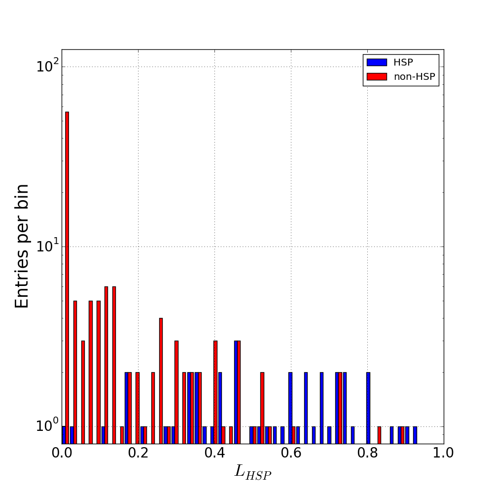
Likelihood distribution of HBL and non-HBL sources in 3FGL blazars by our applied ANN algorithm.
This result could show that the applied algorithm is not able to clearly identify HBLs but the likelihood distribution can still be acceptable for the aim of this study
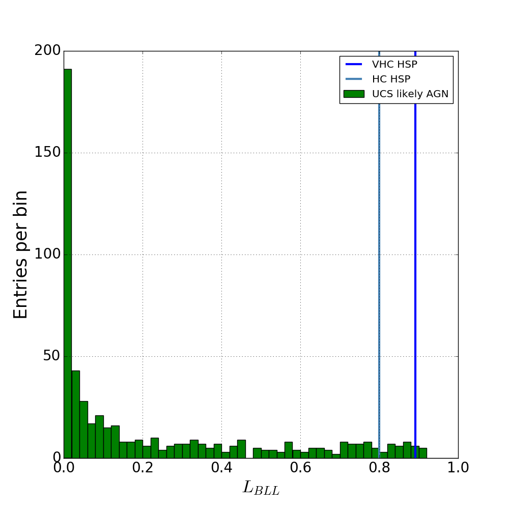
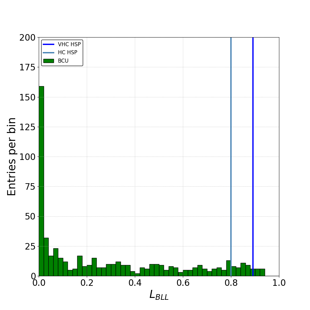
Distribution of the ANN likelihood to be HBL candidates of 3FGL BCUs. (right) and UCS_bcu (left). Vertical blue and steel blue lines indicate the applied classification thresholds to identify sources as High Confidence candidates.
---------------------------------------------------------------------------------------------------------------------------------------------------------------------------------------------------------------------------
Full list of BCU HBL candidates. In Cols. 9, 10, 11 the observabilty at the IACT sites. On the top of the list the candidates with the highest Likelihood (L> 0.89) .
| 3FGL name | Association | TS | Sp.Index | TS_var | L_hbl | RAJ2000 | DecJ2000 | HESS | VERITAS | MAGIC |
| 3FGL J0047.9+5447 | 1RXS J004754.5+544758 | 56.73 | 1.57 | 11.7 | 0.92 | 12.0160498 | 4.80784405 | X | X | |
| X 3FGL J1155.4-3417 | NVSS J115520-341718 | 147.32 | 147.32 | 16.24 | 0.92 | 178.8740215 | -34.32645279 | X | ||
| 3FGL J1434.6+6640 | 1RXS J143442.0+664031 | 73.9 | 1.58 | 16.78 | 0.92 | 218.7228694 | 66.67084133 | X | X | |
| 3FGL J0921.0-2258 | NVSS J092057-225721 | 62.51 | 62.51 | 10.5 | 0.91 | 140.2437951 | -22.94845947 | X | X | X |
| 3FGL J0648.1+1606 | 1RXS J064814.1+160708 | 40.1 | 1.81 | 13.91 | 0.90 | 102.0277929 | 16.08911409 | X | X | X |
| 3FGL J1711.6+8846 | 1RXS J171643.8+884414 | 44.3 | 1.83 | 12.4 | 0.90 | 258.6700448 | 88.75072331 | X | X | |
| 3FGL J1714.1-2029 | 1RXS J171405.2-202747 | 73.8 | 1.44 | 18.16 | 0.90 | 258.5155102 | -20.47598092 | X | X | X |
| 3FGL J1910.8+2855 | 1RXS J191053.2+285622 | 102.25 | 1.61 | 15.16 | 0.90 | 287.7132899 | 28.9403263 | X | X | X |
| 3FGL J0153.4+7114 | TXS 0149+710 | 80.86 | 1.81 | 19.72 | 0.89 | 28.42864335 | 71.25516089 | X | X | |
| 3FGL J0506.9-5435 | 1ES 0505-546 | 455.43 | 1.49 | 29.82 | 0.89 | 76.75704931 | -54.59583993 | X | X | |
| 3FGL J1944.1-4523 | 1RXS J194422.6-452326 | 100.69 | 1.63 | 11.11 | 0.89 | 296.1113217 | 45.38296215 | X | ||
| 3FGL J0742.4-8133c | SUMSS J074220-813139 | 32.29 | 2.03 | 11.8 | 0.92 | 115.4463652 | -81.53829083 | |||
| 3FGL J0040.3+4049 | B3 0037+405 | 75.94 | 1.93 | 12.02 | 0.9 | 10.08708372 | 40.83205536 | |||
| 3FGL J0043.7-1117 | 1RXS J004349.3-111612 | 69.4 | 1.91 | 12.51 | 0.88 | 10.93797337 | -11.31276512 | |||
| 3FGL J1824.4+4310 | 1RXS J182418.7+430954 | 80.91 | 1.82 | 19.74 | 0.88 | 276.1228226 | 43.17807155 | |||
| 3FGL J0528.3+1815 | 1RXS J052829.6+181657 | 35.69 | 1.67 | 14.66 | 0.87 | 82.11289303 | 18.27306451 | |||
| 3FGL J0646.4-5452 | PMN J0646-5451 | 190.34 | 1.46 | 17.37 | 0.87 | 101.6181351 | -54.91863251 | |||
| 3FGL J1959.8-4725 | SUMSS J195945-472519 | 923.79 | 1.51 | 94.31 | 0.87 | 299.9397253 | -47.42901042 | |||
| 3FGL J2108.6-8619 | 1RXS J210959.5-861853 | 91.04 | 1.65 | 10.72 | 0.87 | 316.9856579 | -86.30865936 | |||
| 3FGL J0039.0-2218 | PMN J0039-2220 | 89.34 | 1.66 | 11.61 | 0.86 | 9.766909807 | -22.31500028 | |||
| 3FGL J0305.2-1607 | PKS 0302-16 | 147.6 | 1.6 | 22.94 | 0.86 | 46.29075836 | -16.14465396 | |||
| 3FGL J1040.8+1342 | 1RXS J104057.7+134216 | 69.15 | 1.7 | 11.06 | 0.86 | 160.2594773 | 13.71799931 | |||
| 3FGL J2312.9-6923 | SUMSS J231347-692332 | 35.32 | 1.72 | 16.13 | 0.86 | 348.4026935 | -69.39020448 | |||
| 3FGL J0515.5-0123 | NVSS J051536-012427 | 45.65 | 1.79 | 11.76 | 0.85 | 78.87455087 | -1.419462214 | |||
| 3FGL J0620.4+2644 | RX J0620.6+2644 | 92.02 | 1.53 | 15.1 | 0.85 | 95.17349572 | 26.74390304 | |||
| 3FGL J0640.0-1252 | TXS 0637-128 | 174.15 | 1.52 | 14.44 | 0.85 | 100.0137646 | -12.90013415 | |||
| 3FGL J0733.5+5153 | NVSS J073326+515355 | 104.32 | 1.68 | 11.18 | 0.85 | 113.3491751 | 51.86215575 | |||
| 3FGL J1141.2+6805 | 1RXS J114118.3+680433 | 140.09 | 1.68 | 23.32 | 0.85 | 175.3295357 | 68.0822362 | |||
| 3FGL J1203.5-3925 | PMN J1203-3926 | 103.2 | 1.69 | 18.55 | 0.85 | 180.8463393 | -39.42493679 | |||
| 3FGL J1939.6-4925 | SUMSS J193946-492539 | 64.55 | 1.84 | 15.92 | 0.85 | 294.9560989 | -49.46611442 | |||
| 3FGL J2316.8-5209 | SUMSS J231701-521003 | 37.3 | 1.78 | 15.19 | 0.85 | 349.2774178 | -52.18819115 | |||
| 3FGL J0132.5-0802 | PKS 0130-083 | 71.92 | 1.87 | 12.42 | 0.84 | 23.18651181 | -8.065356912 | |||
| 3FGL J0342.6-3006 | PKS 0340-302 | 43.17 | 1.96 | 13.37 | 0.84 | 55.71024104 | -30.11480314 | |||
| 3FGL J1446.8-1831 | NVSS J144644-182922 | 27.9 | 1.7 | 8.69 | 0.84 | 221.7533056 | -18.51448366 | |||
| 3FGL J1855.1-6008 | PMN J1854-6009 | 21.39 | 1.83 | 6.74 | 0.84 | 283.672544 | -60.1250475 | |||
| 3FGL J0043.5-0444 | 1RXS J004333.7-044257 | 75.94 | 1.91 | 11.93 | 0.83 | 10.8838869 | -4.721385702 | |||
| 3FGL J0746.9+8511 | NVSS J074715+851208 | 118.95 | 1.67 | 18.34 | 0.83 | 117.2491059 | 85.21791595 | |||
| 3FGL J0650.5+2055 | 1RXS J065033.9+205603 | 206.21 | 1.72 | 20.06 | 0.82 | 102.6389899 | 20.92952844 | |||
| 3FGL J1319.6+7759 | NVSS J131921+775823 | 182.64 | 1.95 | 25.12 | 0.82 | 199.9478129 | 78.00731101 | |||
| 3FGL J1908.8-0130 | NVSS J190836-012642 | 306.43 | 2.1 | 35.5 | 0.82 | 287.2015241 | -1.527053471 | |||
| 3FGL J2347.9+5436 | NVSS J234753+543627 | 163.04 | 1.78 | 21.76 | 0.82 | 356.9713227 | 54.58170077 | |||
| 3FGL J0204.2+2420 | B2 0201+24 | 27.62 | 1.7 | 12.29 | 0.81 | 31.09102234 | 24.27132207 | |||
| 3FGL J0439.6-3159 | 1RXS J043931.4-320045 | 119.86 | 1.74 | 24.96 | 0.81 | 69.85155048 | -32.03484089 | |||
| 3FGL J1547.1-2801 | 1RXS J154711.8-280222 | 96.77 | 1.77 | 16.75 | 0.81 | 236.8077415 | -28.04443418 | |||
| 3FGL J1612.4-3100 | NVSS J161219-305937 | 494.96 | 1.86 | 116.18 | 0.81 | 243.1006458 | -30.99149787 | |||
| 3FGL J0030.2-1646 | 1RXS J003019.6-164723 | 168.7 | 1.66 | 30.18 | 0.8 | 7.586848013 | -16.82218924 | |||
| 3FGL J1158.9+0818 | RX J1158.8+0819 | 51.45 | 1.81 | 11.81 | 0.8 | 179.7088941 | 8.311328097 | |||
| 3FGL J1841.2+2910 | MG3 J184126+2910 | 195.91 | 1.79 | 22.89 | 0.8 | 280.3558247 | 29.15522239 |
--------------------------------------------------------------------------------------------------------------------------------------------------------------------------------------------------------------------------
Full list of BCU HBL candidates. In Cols. 8, 9, 10 the observabilty at the IACT sites. On the top of the list the candidates with the highest Likelihood (L> 0.89)
| 3FGL name | TS | Sp.Index | TS_var | L_hbl | RAJ2000 | DecJ2000 | HESS | VERITAS | MAGIC |
| 3FGL J2142.6-2029 | 36.07 | 1.68 | 8.19 | 0.914 | 325.6572 | -20.4955 | X | X | X |
| 3FGL J2321.6-1619 | 34.14 | 1.73 | 45.13 | 0.911 | 350.3966 | -16.3171 | X | X | X |
| 3FGL J2145.5+1007 | 52.53 | 1.70 | 19.90 | 0.906 | 326.3815 | 10.1296 | X | X | X |
| $3FGL J2300.0+4053 | 174.53 | 1.64 | 6.97 | 0.904 | 345.0583 | 40.8750 | X | X | X |
| 3FGL J2224.4+0351 | 29.5 | 1.93 | 9.55 | 0.89 | 336.1020 | 3.8590 | |||
| 3FGL J1525.8-0834 | 59.52 | 1.92 | 23.26 | 0.89 | 231.4700 | -8.5790 | |||
| 3FGL J1619.1+7538 | 107.12 | 1.86 | 14.91 | 0.88 | 244.9610 | 75.6730 | |||
| 3FGL J0251.1-1829 | 104.26 | 1.58 | 10.20 | 0.88 | 42.7970 | -18.4860 | |||
| 3FGL J0020.9+0323 | 60.66 | 2.09 | 22.50 | 0.88 | 5.2310 | 3.3950 | |||
| 3FGL J0813.5-0356 | 57.02 | 1.71 | 13.15 | 0.88 | 123.3870 | -3.9390 | |||
| 3FGL J1234.7-0437 | 51.54 | 2.00 | 29.76 | 0.87 | 188.6970 | -4.6220 | |||
| 3FGL J1922.2+2313 | 80.83 | 2.22 | 22.63 | 0.87 | 290.5650 | 23.2260 | |||
| 3FGL J2043.6+0001 | 48.48 | 2.01 | 24.43 | 0.87 | 310.9010 | 0.0290 | |||
| 3FGL J0312.7-2222 | 177.14 | 1.84 | 18.27 | 0.87 | 48.1760 | -22.3710 | |||
| 3FGL J1513.3-3719 | 54.74 | 1.91 | 18.06 | 0.87 | 228.3290 | -37.3190 | |||
| 3FGL J0524.5-6937 | 94.15 | 2.05 | 18.37 | 0.86 | 81.1280 | -69.6290 | |||
| 3FGL J1225.4-3448 | 22.27 | 1.74 | 7.01 | 0.86 | 186.3560 | -34.8070 | |||
| 3FGL J1222.7+7952 | 43.83 | 2.12 | 14.79 | 0.86 | 185.9965 | 79.8921 | |||
| 3FGL J2309.0+5428 | 77.06 | 1.75 | 17.68 | 0.85 | 347.2520 | 54.4760 | |||
| 3FGL J2015.3-1431 | 17.42 | 1.81 | 14.63 | 0.85 | 303.8543 | -14.5344 | |||
| 3FGL J2053.9+2922 | 359.63 | 1.76 | 43.97 | 0.85 | 313.4760 | 29.3740 | |||
| 3FGL J0234.2-0629 | 90.7 | 2.00 | 20.73 | 0.84 | 38.5640 | -6.1050 | |||
| 3FGL J1545.0-6641 | 150.1 | 1.59 | 11.85 | 0.84 | 236.2650 | -66.6997 | |||
| 3FGL J0731.8-3010 | 37.07 | 1.96 | 12.91 | 0.84 | 112.9740 | -30.1770 | |||
| 3FGL J0952.8+0711 | 50.96 | 1.91 | 14.12 | 0.84 | 148.2170 | 7.1990 | |||
| 3FGL J0527.3+6647 | 51.89 | 1.90 | 14.78 | 0.83 | 81.9000 | 66.7767 | |||
| 3FGL J1528.1-2904 | 26.28 | 1.80 | 11.72 | 0.83 | 232.0360 | -29.0680 | |||
| 3FGL J0049.0+4224 | 36.95 | 1.80 | 16.58 | 0.82 | 12.2530 | 42.4130 | |||
| 3FGL J1057.6-4051 | 40.23 | 1.71 | 15.54 | 0.82 | 164.4090 | -40.8620 | |||
| 3FGL J0928.3-5255 | 98.75 | 2.09 | 26.68 | 0.8 | 142.0300 | -52.8680 |
-----------------------------------------------------------------------------------------------------------------------------------------------------------------------------------------------------
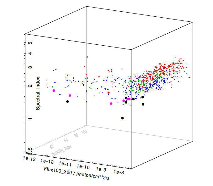
The 3D plot shows the distribution of HBL candidates against the 3FGL blazar subclasses HBL [blue], IBL [green] , LBL [ red ].
All the candidates lie in the clean HBL area validating the ANN results that classified the target as HBL sources.
TeV candidates
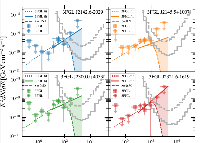
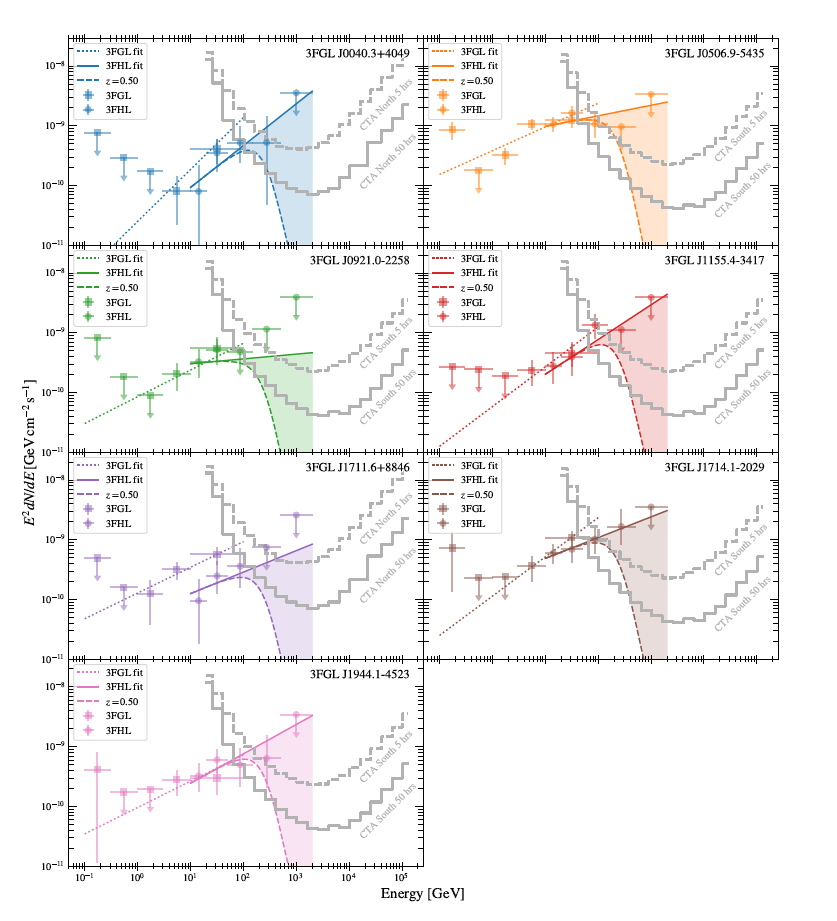
We compare the extrapolated fluxes of the candidates against the sensitivity of present IACTs and the future CTA. We used the Fermi-LAT spectral shape of the sources obtained in the range between 0.1 and 300 GeV using the best-fit model parameters from the LAT 4-year 3FGL Catalogue and particularly we referred to the spectral model that fits the data.
We compare the extrapolated fluxes with the CTA sensitivity for 50 hours (5hours) of observations as a solid (dashed) grey line.
Above a declination of 0 degrees we use the sensitivity of the northern array and the southern array otherwise.
The CTA sensitivity for 5 hours of observations is similar to that of currently operating IACTs for 50 hours of observations except a higher threshold energy of ~ 80 GeV.
52 Comments
-

AGN group science coordinators comments on HBL_aa_VP_approved version below:
There are some main general points that at the moment make the project a bit weak (it is nothing seriously wrong but just a warning that the referee might find the paper not very impactful):There is some confusion whether you are primarily searching for HSP sources or TeV candidates. The two things are to some extent overlapping but if the ultimate goal is to find TeV candidates, having an HSP classification is surely not enough, because the Fermi flux is another very significant constraint. The combination of these two requirements results in a very low efficiency of the method: starting from a sample of over 1100 sources, it seems you select only 15 good candidates (Table 3), many of which will not be detectable above fairly low values of redshift anyways (see below a caveat on the assumptions about redshift, too).On the other hand, if the goal is "simply" to classify HSP sources, it would be good to compare the performance of the method with respect to other tools, for example the value of the gamma-ray photon index which is generally readily available and is also expected to be a good (better?) proxy for HSP-ness. And again, if you want to also consider the possibility to later detect the sources with CTA/IACTs, the extrapolation of the Fermi SED, as you show in this paper, too, is of critical importance.The last more general concern is the applicability of the method to future catalogues: since the ANN method is based on light curves, it seems that it is best applied to sources bright enough to be detected on relatively short time intervals. For this reason it is probably of little use for sources that will become detected in future catalogues only thanks to longer exposures.Besides these, please find below a few more points, mostly minor/editorials but still useful to improve the paper quality:- line 20: "by the presence of many competing" —> "with" (the presence of competing populations is not specifically a limitation of IACTs - it is its combination WITH the small field of view that makes it a limitation)- line 25: "50 hours" —> "for a given exposure time" (the method is quite general and you do not need to specifically define the duration here - also because 50 hr with current IACTs and with CTA will deliver significantly different results)- line 42-43: sensitivity goes with t^(-1/2) so it would make more sense to be more accurate on the flux than on the time; please specify how much is "a few"- lines 57-59: I would expand a little bit the introduction of the three SED types LSP-ISP-HSP. It is ok to quote the reference to the paper where the three classes where defined. In addition, I would explicitly recall the big effort, particularly in the 3LAC, where a team of "SEDders" visually inspected each LAT blazar and performed and SED fitting to obtain the peak frequency and hence the classification of the source. This is where you get the classifications to train your method in the first place.- line 62: 48+7 is still a minority population with respect to 211, maybe you could quote (in parentheses or perhaps in a footnote) that the rest of the population is of galactic or even unidentified nature- line 64: define WHSP- line 74/75: please reword the sentence between "50% and UCSs"; the current meaning is not clear- line 80: an "s" escaped from the subscript UCS_agns- figure 1: since the paper is about the selection of HSPs, it would make more sense to show the histogram for HSPs vs non-HSPs rather than for BLLacs vs FSRQs- line 114: a —> an- figure 2: I wonder if showing, eg, the cumulative distribution would not be a more effective way to show the strong difference between the two populations. It seems the main point here is that it is really hard to achieve high L_HSP values for non-HSP sources, so maybe showing a normalised, or a cumulative distribution, and maybe using a linear y-scale, would show better how the overwhelming majority of the non-HSP sources are at low or null L_HSP. Not sure it will help but it could be worth experimenting.- lines 116-123: I don't seem to find the description of the results on the testing sample. I think this should be given. Or maybe I'm confused by the structure and this is given in the next section in lines 129-137. If that's the case, I strongly suggest to move all this part back to the end of section 2.- why do you mention a precision of 90% in l. 133 and then it becomes 75% in l. 135?- line 145: put the whole Chang reference in parentheses- line 152: what do you mean by "best"?- line 158: put the whole Acero reference in parentheses- line 166: why did you use a square RoI in place of the usual circular one?- line 176: it would be interesting to see how your calculated TS_VAR compares to the variability index reported in the 3FGL- line 180: add "…, respectively" at the end of the sentence.- line 194-195: this is a very open and long standing debate in which many people argue that the BL Lacs without a redshift are likely much more distant than those with a measured one. Padovani, Giommi & Rau 2012 is probably a good starting reference on this. I would add a caveat that some objects could fall beyond the 0-0.5 redshift range.- line 197, 209 (and please check elsewhere): here the HC_HSP sample becomes HC_TeV. This goes back to the initial general comment about confusion between looking for HSPs or TeVs. I would stick to HC_HSP throughout the paper.- footnote 5 and Figs 5-6. I'm a little concerned about the CTA sensitivity curves. In the energy range above 1 TeV, it looks like there is an increase of nearly an order of magnitude when going from 5 to 50 hours of observations. I would naively expect an improvement of a factor sqrt(50/5)~3.2 or so. Do you have an explanation for that? Sorry if I should know better myself.- Table 2: please quote only 1 digit after the decimal point for TS and TS_VAR, and make sure that trailing zeros appear in the spectral index column. -
Dear AGN group science coordinators, thank you for your precise and careful revision of the paper. I will pay close attention to your comments and I'll improve of the paper, with a new version.
-
Dear Graziano, please find below a few very minor editorial comments on the latest version (HBL_aa_MArev2_DJT1).
line 67: here you have catalog while elsewhere you use catalogue
line 91 - put Salvetti et al. out of parentheses
line 96, 107, 115 - same for Chiaro et al.
line 130: replace "BL Lacs and FSRQs" with "HSPs and non-HSPs"Green light from AGN coordinators.
-
Dear authors,
I'm reading v(HBL_aa_MArev2_DJT1) on behalf of the publication board. I think this is a nice result, I have a few comments on to help the clarity on some of the points.
Overall: Figures 1-3 need to have larger legends and Fig 1 needs larger axis labels.
19: "Observations by IACTs...": I think the important thing to emphasize here would be the importance of weighting targets since observation time is limited on IACTs in general.
22: "The aim of this paper...": Is the unclassified blazar population here the unclassified Fermi-LAT blazar population? I would be specific.
34: Are blazars the most powerful AGN? Or are they a type of AGN?
50: It sounds here that it was the 3FHL that selected TeV-telescope candidates instead of the candidates being selected from the 3FHL
54: I think regardless of the units of the SED there are two broad humps for AGN. I would probably end the sentence at "broad humps"
76: One of the steps in the approach is to look for variability, but you don't state the expectation (or motivation)
89: I would put the references at the end of the sentence for readability.
97: "extragalactic TeV-energy sources" - do you mean targets? (currently not TeV sources)
104: I would modify the title from "The search method" (which is quite generic) to specifically the search method you're using maybe "The AAN technique" or something like that
105: a perceptron is a term specifically for NNs. I would take an additional sentence or two to define what it is. Maybe even a figure.
109: Can you state the parameters you're using to train the algorithm?
115: In your training algorithm, did you also give it the option to classify something as "not an AGN". In the case that a pulsar accidentally got thrown in there?
129: Since Fig 1 is only demonstrating that the variability index isn't an important parameter - you can probably remove it (I think a figure of a generic NN technique would be much more useful).
152: "cleanest" -> best?
Figure 4: I'd break this into multiple figures. The 3D looks really cool, but it's hard to see what's happening on the variability index axis.
165: I'd be explicit here and say what exactly the algorithm is able to find
167: "We performed an analysis of Fermi-LAT data analyzing 104 months of Pass 8 data, from..." This is a really long sentence with a lot of ideas. you can probably condense it a bit here "We analyzed 104 months of Fermi-LAT Pass 8 data from....."
197: It seems like the spectral indices for HSPs/LSPs and ISPs are consistent within uncertainties?
205: a lot of the discussion of the EBL probably isn't needed here. The sentence in particular that state "The relevant part of the EBL..."
236: Conclusion -> Conclusions
-
Here are some comments for your consideration based on the PubBd version 4 of the paper.
38: citations for MAGIC, HESS, VERITAS, CTA are missing
47: please cite the LAT instrument paper (Atwood, W. B., Abdo, A. A., Ackermann, M., et al. 2009, ApJ, 697, 1071) instead of the 3FGL paper (which is introduced and cited at line 81)
121: I'd be curious to see some examples of the cumulative percentage as a function of flux. Are there any on confluence ? It's certainly beyond the scope of the paper, but it seems to me that looking at these curves for HSPs and LSPs might help you to understand why/how the quantiles variables are good variables to discriminate between them. Without having seen these figures, I'd guess that there might be a way to fit them with some functional form with a couple of parameters. I would not be surprised that feeding the ANN with these parameters would do a similar good job, and maybe would help to improve the performance.
129 and caption of Fig.1: we found the Variability Index to be, in our algorithm, an unimportant parameter. I think that this statement is not fully correct. What is correct is to say that using the Variability Index on top of the quantiles does not improve the performance. Fig.1 shows that it is not possible to use the Var Index alone as a discriminating variable, but Fig.4 shows that it can be useful when used with other variables.
135: remaining -> the remaining third (?)
Fig.2: which sample do you use (I assume it is the testing sample)? I see ~44 HSP entries while I expect 289/3=96 entries.
162: All the candidates... Personal comment: if the selected HSP candidates all lie in a clean HSP area and far from the LSPs, it seems to imply that you could define a clean selection based on these 3 variables and that your ANN approach is not much more powerful than a simple 3D cut in that space.
168: please cite the Pass 8 paper: Atwood, W., Albert, A., Baldini, L., et al. 2013, eConf C121028, 8, in Proc. 4th Fermi Symposium, Monterey
169: zmax cut ?
In the printout version, the bottom of Fig.1 and the top of fig.2 are missing. I don't know whether it is a sign of something wrong with the figures.
-
Thank you Philippe for your useful comments , I'll adjust the text and I'll post the new version.
Concerning your comment at line 121 please consider the following text.
Much of the proposed ANN method and examples of cumulative percentage as function of flux in order to show how the adopted parameters are good discriminators are described in https://arxiv.org/pdf/1607.07822.pdf
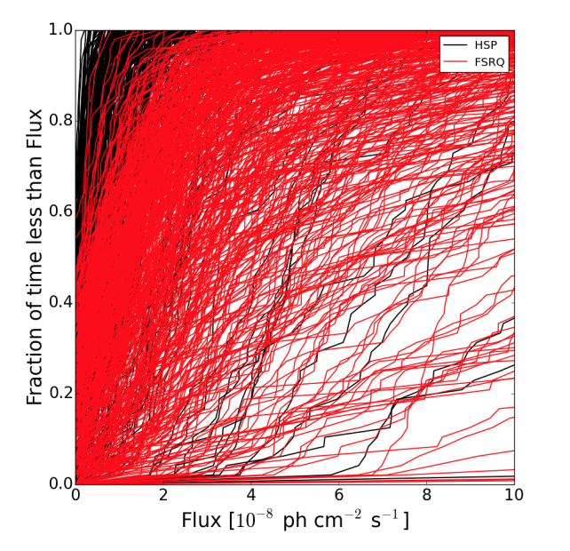
The original idea was to compare the γ-ray light curve of the source under investigation with a template classified blazar class light curve, then measure the difference in a proper metric. Typically γ-ray AGN are characterized by fast flaring that could alter significantly the light curve and could make the comparison difficult. In addition, different flux levels could hide the actual similarity of light curves. As first approach of the ANN study we computed the Empirical Cumulative Distribution Function (ECDF) of the light curves. We constructed the percentage of time when a source was below a given flux by sorting the data in ascending order of flux in order to compare the ECDFs of uncertain blazars with the ECDFs of blazars whose class is already established. This was our variation of the Empirical Cumulative Distribution Function (ECDF) method. Fig. 1 shows the ECDF plots for 3FGL BL Lacs ( blue) and FSRQs ( red) . Fig.2 shows the significant overlap between the types where it is hard to distinguish individual objects, and there are outliers that extend beyond the range of the plots, but it is possible to recognize on the top left of the diagram a specific area where the overlap between BL Lac and FSRQ is minimal that , could lead to a first qualitative recognition of BL Lac objects. Because the aim of the studies was to quantify the likelihood classifying an uncertain source we used the a two-class ANN algorithm.
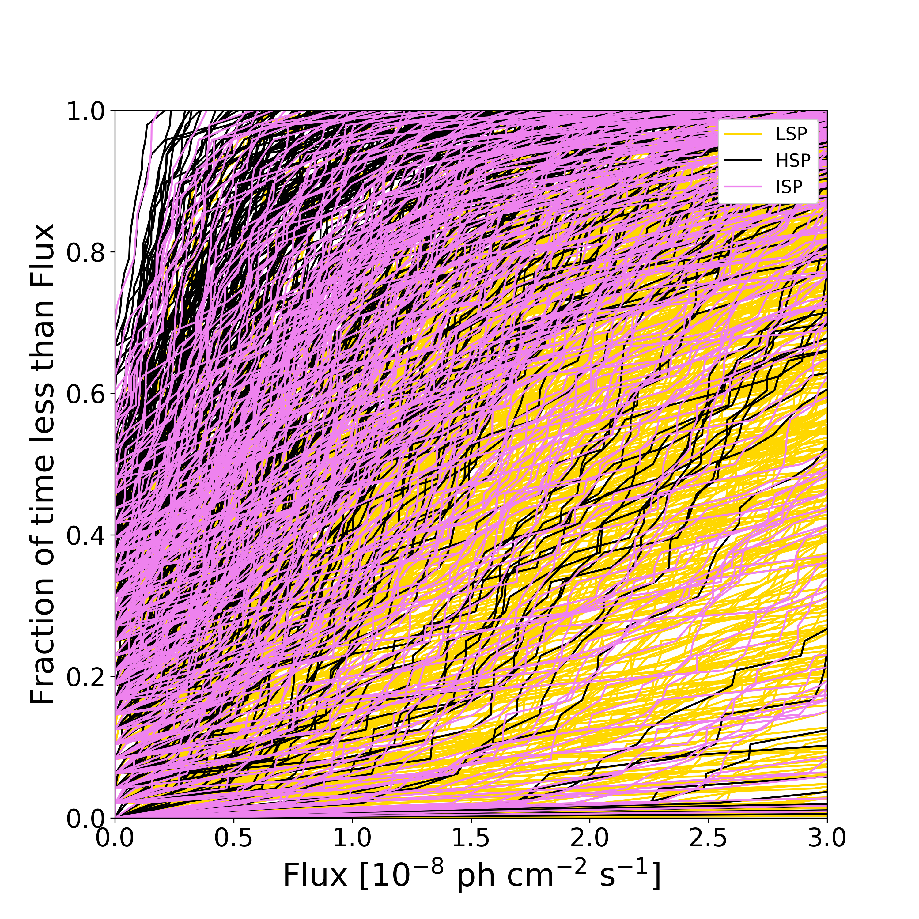
Following the procedure used for blazars we applied the algorithm to the blazar subclasses even if the ECDF results weren’t not as satisfying as for the blazars. However a clean area where to apply the ANN was found as described in the paper. Fig. 3 shows the ECDF for blazar subclasses, where the HSP( black) / FSRQ( red) separation is evident, but when we considered the blazar subclasses the HSP / LSP separation was also evident but the ISP contamination was not negligible. However applying the ANN the results proposed in this paper are consistent and acceptable. Even if it could be possible to consider different parameters than flux variability the aim of this and previous studies is to characterize the sources by their γ-ray light curve. However, experimentation with new parameters continues to verify the possibility to obtain new specific algorithms applicable to the new Fermi AGN catalogs.
Best regards
Graziano
Fig.1
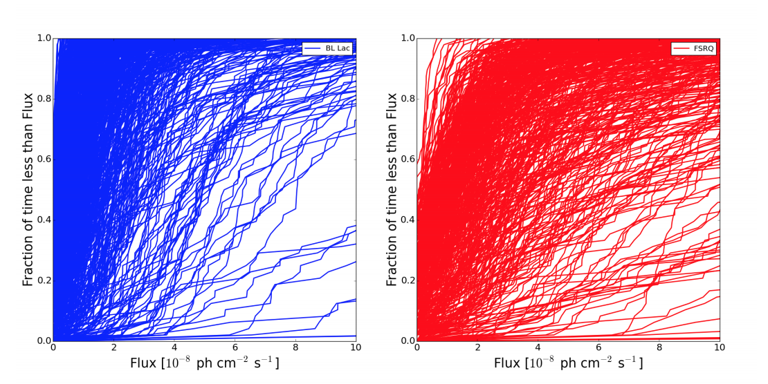
Fig.2
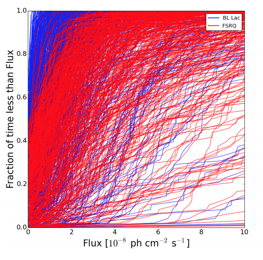
Fig.3
-
Philippe,
about your comment for :
_ Fig.2 _ Yes , that's the plot of the testing sample optimizing the ANN algorithm
- Fig.4
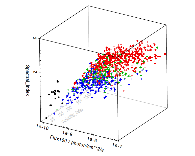
Your are right when you comment that it could define a clean selection based on these 3 variables , but please conside that our algorithm is a two parameter / two layer algorithm and we could not have used three parameters
Best regards
Graziano
-
Thanks Graziano. Regarding fig.2, as I said, I expect 289/3=96 HSPs but it seems that there are only ~44 HSPs. Am I missing something ?
- Fig.4
-
Hi Philippe,
I talked with David Salvetti who made the plot in Fig.2 and he confirms that 1/3 of the total sample was in the plot. I don't have the full list of sources and related likelihood right now on my notebook, but however the aim of the plot is to show that there are much more LSP/ISP than HSP and these latter sources has no clean peak in order to show also in the ANN plot the ISP ( and LSP) contamination that we saw in the ECDF plots.
I tried to count the entries, looking by eyes the plot. It seems to more than 40 sources( ~ 60? ) but I think that the plot could be fine for the aim of this study. It could be possible to repeat the plot but it means to analyze once more the whole sample and this is not a fast work. Is it okay for you?
Best
Graziano
-
No, I haven't because we considered HSP and non-HSP sources ( ISP +LSP). We have separate colours in the ECDF plot as I posted above in Fig. 3. Also plot red/black in Fig.3 is interesting if you consider that FSRQs are mainly LSP objects.
-
No, I'm sorry Philippe, we haven't any separate diagram because owe used a the two class algorithm that considers the likelihood A = 1-B then it returns an histogram with both the likelihood as you see here in Fig.2 . The most interesting result was to compare the two " classes" together as did for BL Lac vs FSRQs likelihood. However the two selection are easy readable in the histogram.
-
I'm very surprised that you haven't stored the ANN results of the test sample and that it could take a long time just to just reproduce the plot. In my opinion, the bin size is too small and it's not clear whether the non-HSP histogram hides part of the HSP histogram. I think that this figure is key to the analysis and I think that the reader can expect to be able to see the full HSP distribution. Since I don't see the 96 entries, I can't say that I see the full distribution.
-
-
Thank you Philippe of your comment. Let me talk with my colleagues and I'll answer to you as soon is possible.
-
Hi Philippe,
All the commented minors have been reviewed and adjusted.
According with your suggestion, in order not to creare confusion in the reader, Fig .4 and the relative text were deleted because they did not add any extra value to the ANN result.
Moreover I reviewed all the ANN data and I can answer your comment
“… Regarding fig.2, as I said, I expect 289/3=96 HSPs but it seems that there are only ~44 HSPs. Am I missing something ? ”
A mistake was made writing the text of the paper you reviewed. Instead of testing test, training test was written. The correct wording is testing test. Therefore the percent of samples used for the testing sample is different. The testing test accounts for 15% of the total sample. In this way Fig. 2 is correct (~ 43 HSPs and ~ 123 non-HSPs). The relating text has been re-written and highlighted in blue in the new draft posted in PubL Board.
Graziano
-
Thanks Graziano for the clarification/correction.
Minor comment:
133: that represent of -> that corresponds to
-
-
Hi Graziano,
It looks like you've addressed Philippe's comments with the newest upload to the pubboard. Can you confirm that you took into account my comments?
Thanks!
Best,
Regina-
Hi Regina,
I didn't see any comment from you before your last post.
When did you comment?
Graziano
-
-
Hi Regina,
sorry for late reply. I reviewed the paper considering also your precious comments. A 2LP ANN schematic figure has been added to the paper. About your comment concerning a pulsar contamination of the sample, it remains free of pulsar because the 559 UCSagn objects came from a previous Pablo Saz Parkinson study (Saz Parkinson et al. 2016 https://arxiv.org/abs/1602.00385) where Pablo applied a number of statistical and machine learning techniques to classify and rank unclassified gamma-ray sources in 3FGL as UCSagn and UCSpsr.
Best
Graziano
-
Dear co-Authors and Publ Board.
I received the referee report and I post it here.
-
Referee report
Main comments:
The manuscript with title “Identifying TeV source candidates among Fermi-LAT unclassified blazars using Artificial Neural Networks” by Chiaro et al. reports the results of using artificial neural networks (ANN) to identify promising High Synchrotron Peak (HSP) candidates among the 573 3FGL blazar candidates of uncertain type (BCU) and among 559 3FGL unidentified sources likely to be blazars. It also reports the analysis of 104 months of Fermi data for the 80 selected HSP candidates and the comparison of corresponding extrapolated spectra with the sensitivity curves of present and future IACTs.
Finding new TeV blazar candidates (not only HSPs) is important, not only for the study of acceleration/radiation mechanisms in AGN, but also to make possible blazar population studies at these energies. As very long exposures are often needed to detect TeV emission, to provide such a list of TeV HSP candidates is of interest to the community. The Fermi analysis work performed by the authors on these 80 HSP candidates also deserves publication.
However, the manuscript cannot be recommended for publication in its current form.
The main issues are:
• The ANN search method presented in Section 2 seems to be exactly the same as the one published in Chiaro et al. 2016 (see sections 3 and in particular 3.3 in Chiaro et al. 2016). It is presented here (L. 116) as an optimized version of the one in Chiaro et al. 2016, but it seems that no changes have been made. Indeed, the distribution of L_HSP in the testing sample and the thresholds used to select HSPs are exactly the same in both papers. In particular, figure 3 in the present paper has already been published as figure 7 in Chiaro et al. 2016. Surprisingly, the results of the application of the ANN algorithm to the same selected 573 BCUs differ between both papers (48 HSP candidates are found here with L_HSP>0.8 and 11 with L_HSP>0.891, whereas 53 with L_HSP>0.8 and 15 with L_HSP>0.891 are published in Chiaro et al. 2016). This must be clarified.
• The presentation of the ANN method and its limits are not detailed enough, neither in the present paper nor in that of 2016 (for HSPs):
o In particular, the authors have to handle with small datasets, which imply that the variance of classifiers corresponding to random training/validation/test splittings is likely to be important. Consequently, a single random training/validation/test splitting will provide a performance that could be significantly misestimated. An illustration of the fragility of the ANN performance presented in the paper is visible in figure 3, with only 1 or 2 true HSPs (and 0 or 1 non-HSP) in the testing sample passing the high confidence HSP cut (L_HSP>0.891). Authors should discuss this. For optimization purposes, in particular when dealing with small datasets, 10-fold cross-validation is a standard that has been previously used in similar works (train the classification method on 9/10ths of the training sample and apply it on the remaining 1/10th, then repeat ten times until the whole training sample has been tested on once, and derive performance metrics from there). Using 70% of the!
3LAC HSps and ISP-LSPs for 10-fold cross-validation would allow using the remaining 30% as testing sample (instead of 15%). It would be interesting also to use receiver operating characteristic (ROC) curves (see, e.g., Fawcett, T, Pattern Recognition Letters, 27 (2006) 861-874) to check the stability/variance of performance due to the small samples size (see how Lefaucheur et al. 2017 A&A 602 86 dealt with this problem).
o It is difficult to understand why only variability information is used to build classifiers for HSP / non-HSP identification. It has been shown that additional separation power between BLLs and FSRQs (and so between HSPs and FSRQs, as most HSPs are BLLs) is carried out by other parameters provided by the 3FGL catalogue (see Ackermann 2015 for the 3LAC spectral properties, and similar works dedicated to the separation of different type of blazars: Hassan et al. 2013 MNRAS 428, 220–225; Lefaucheur et al. 2017 A&A 602 86; etc.).
o It is obvious that the choice of building an ANN method on flux-dependent information can imply that ANN performance is also flux dependent. Did the authors compare the flux distribution for HPSs, ISP-LSPs, BCUs and UCSagn? How the upper-limits in the month light-curves were treated?
o Other authors (see Lefaucheur et al. 2017 A&A 602 86) have shown the importance of taking into account the analysis flags in 3FLG catalogue to reach a proper derivation of classifiers performance. Maybe this issue is less important here, where classifiers are built only on flux variability, but this should be evaluated. What are the fraction of sources with analysis flag for HPSs, ISP-LSPs, BCUs and UCSagn?
o The estimation of the number of false identifications among the HSP candidates is missing. Please give it explicitly. The expected number of false identifications should be considered separately for HSP candidates from the BCU and from the UCSagn samples. This is particularly delicate in the case of UCSagn because of how the sample of 559 sources has been obtained (from Saz Parkinson et al. 2016 and not from Salvetti et al. 2017 as reported in the present paper). Indeed, beyond the fact that Saz Parkinson et al. 2016 didn't provide an estimation of the number of false identifications, their classifiers were built to identify sources as pulsars or AGN not taking into account the presence of SNR and PWNs close to the Galactic plane. They didn't take into account the effect of flagged sources on their classifiers performance, whereas 3FGL low galactic latitude sources are dominated by flagged sources. For these reasons, it is likely/possible that there is a significant amount!
of false identifications among the low galactic latitude blazar candidates of Saz Parkinson et al. 2016. I recommend to limit the present study to the 481 (instead of 559) Saz Parkison et al. 2016 blazar candidates with galactic latitude above 10° (|b|>10°).
o Do the authors understand why in Fig. 3 there is not a peak at L_HSP~1 ? Please add a comment.
• This paper reports the analysis of 104 months of Fermi data for the 80 selected HSP candidates. Therefore, the results of these analyses should be reported in Tables 1 and 2 in a much more complete manner: spectral index with its error, pivot energy, flux at the pivot energy with its error, etc., should be provided. These results are of interest as they could be used for different physics cases in the gamma-ray community.
• It seems that Fermi spectra are obtained for an energy range starting at 100 MeV. As shown in the 3FHL paper, the average difference of photon indexes for spectra starting at 100 MeV and spectra starting at 10 GeV is about 0.3-0.4 (for redshifts in the 0-0.5 range). As spectra starting at 100 MeV tend to be harder than spectra starting at 10 GeV, their extrapolation at higher energies will tend to be overoptimistic for detections with IACTs. Could the authors make a comment about that?
• There is an issue in the comparison of Fermi extrapolated spectra with CTA sensibility. It makes sense to consider the observation with the northern (southern) array of sources with declination above (below) 0°. But as the CTA sensitivity varies with the observation zenith angle, the CTA consortium provides sensitivity curves at 20° and 40° zenith angles for each array. Considering the latitude of the arrays (+28° for the northern array, -24° for the southern array), the authors should select for each source the more appropriate sensitivity curve and explain it in the text (L213-214). Figure 5 shows that, for a given array, the authors used the same sensitivity curve whatever the source declination. The HESS, MAGIC and VERITAS columns in tables 1 and 2, and the zmax columns in table 3 must be updated correspondingly.
• Finally, the abstract, a part of section 1 (second part of the third paragraph) and almost all the section 2 are far to be in an acceptable shape and need to be re-read by all the authors (obviously this was not done). In addition, section 2 must indicate that the description of the ANN method is already given in Chiaro et al. 2016 and that there is no further optimization here.
If the authors address the above-mentioned issues, the resulting HSP-candidates list and the analysis work performed on Fermi data are of interest for the community and would deserve publication.
Additional (less important) comments are listed below.
Other comments:
Abstract
L16: replace "are the main targets" with something like "are among the main targets".
L23: CTA is also an IACT. Replace by “the present IACTs or the future CTA”?
L22-26: it is a vague summary of the work done in the paper. Please improve it (many key-words missing: HSP, 3FGL, BCUs + blazar-like unidentified sources, 104 month of Fermi data) and be more precise on the results.
L28-30: weak affirmations => to be removed (otherwise please provide a justification in the text).
Section 1: Introduction
L34: The reference Abdo et al. 2010 refers to the paper “Suzaku Observations of Luminous Quasars: Revealing the Nature of High-Energy Blazar Emission in Low-level activity States”. Is it an error?
L48: Please explain why the 3FHL catalogue is interesting to searching for TeV blazar candidates (and fix the typo).
L48-49: Is this sentence referring to the 3FHL paper also?
L50: "alternative". I don't really see where is the alternative. In all cases it is necessary somehow to compare the spectral properties in the gamma regime with IACTs typical capabilities.
L59: The Abdo et al. 2010 reference is not the correct one. If the authors are referring to the 1LAC paper, please fix de reference.
L61-73: The end of this paragraph is not well written in its current form. A few examples: not clear in L61-63 if the work of these SEDders is for 3LAC or not; the sentences about TeVCat do not clearly illustrate that HSPs are the most numerous sources in the TeV extragalactic sky – the authors could try: “Indeed, in the TeVCat interactive catalogue for TeV sources (Horan et al. 2008), among XXX extragalactic sources XXX are HSP, while...” etc.; the link between the part about 2WHSP and previous lines is not obvious. Please clarify.
L65: The VHE regime is usually defined as gammas above 100 GeV, as in Chiaro et al. 2016... the definition used in the TeVCAt proceeding is not usual.
L66-67: TeVCat numbers are not up to date. Please fix this. There is something wrong about LSP/ISP and FSRQs. Note that in TeVCat, the LSP/ISP classifications are not used, but rather LBL/IBL. I see in TeVCAT 49 HBL, 8 IBL, 2 LBL and 7 FSRQs. There is a typo in footnote 7 (missing "of")
L74: Please replace "TeV source" by "TeV HSP"
L74-76: Please be more precise. The HSP candidates are not searched for among all the unclassified Fermi sources; the first part of the work is performed on the basis of 3FGL information.
L80: Is it 3033 or 3034?
L87: Space missing before "("
L88: Typo: Leufaucheur => Lefaucheur
L89: Not Salvetti et al. 2017, but rather Saz Parkinson (2016) !
L91-92: “We focus on […]”. The authors should cite previous similar works: Hassan et al. 2013 on the 2FGL catalogue, Lefaucheur et al. 2017 on the 3FGL catalogue.
Section 2: the ANN search method
Fig. 1: Too general and not very informative, already published in Chiaro et al. 2016. Please remove.
L104: Reference required for such a statement.
L107-145: The content of this section has already been published in Chiaro et al. 2016. The version proposed here is much less well-written (typos, repetitions, sentences difficult to understand, etc.). Please see the “Main comments” section.
Fig. 2. The figure does not bring interesting information. Despite the important overlap between the distributions, discrimination power of this parameter could be hidden in the correlations with other parameters. In addition, it is preferable to avoid the "direct use of variables correlated with the overall flux" (see Doert and Errando 2014). Anyway, the distributions should be normalized, and labels and units are too small.
L131-132 and elsewhere: It’s worth to indicate that by non-HSPs sample the authors mean ISPs and LSPs (from 3LAC and not from 3FGL, I guess).
Fig. 3: Fix the typos. Please specify that non-HSP sources are ISP and LSP in the 3LAC catalogue.
Section 3: Identifying HSP candidates
L147: Remove “optimized”
Fig. 4: In both figures, please fix the thresholds names: “HC HSP threshold” instead of “VHC HSP”; “HSP threshold” instead of “HC HSP”;
L149-150: A comment about the absence of peak at L_HSP ~1 would be nice here.
L153: In section 2, a threshold is defined corresponding to a precision of 90% (true positives/(true positives + false positives)). In section 3 it is mentioned that the L_HSP>0.891 threshold corresponds to a true positive ratio (true positives/positives) of 90%. Are the authors referring to the same threshold? Please clarify.
Table 1 and 2:
Please specify what “observability at IACT sites” means. What observation time is considered? A column for CTA observability is missing.
As the HC cut is at L_SHP>0.891, please add a digit in the L_HSP column and also in the captions. In table 2, the 3 sources with L_HSP=0.89 are they all below 0.891 as suggested by the horizontal line?
In table 2, what do the symbols before some of the 3FGL names mean?
Section 4: Fermi-LAT spectral analysis
L159: typo: from from
L176: The normalization and slopes of the IEM and isotropic templates were allowed to vary during the fit. Could the authors make a comment about possible deviations with respect to the starting values?
L188-189: Where the reported values come from, in particular for LSPs and ISPs? Have the authors performed also an analysis of LSPs and ISPs for the same period? Please clarify.
Section 5: TeV candidates
L203-204: note that z=0.022 is reported for the source 3FGL J0153.4+7114 (seen in Simbad, I didn’t check its reliability).
L204: Especially true for HSPs, not for all types of BL Lacs (see fig. 12 in the 3LAC paper)
L205: “these z values” => “these two z values”
L213-214: see the “Main comments” section.
Figures 5 and 6: far too small.
Section 6: Conclusions
L236-238: I don’t understand this “the very similar values of the synchrotron peaks of the three blazar subclasses”… the synchrotron peaks positions are spread over orders of magnitude and are, by definition, different for the different subclasses. Please rephrase.
General:
Remove spaces before footnotes-
In light of the extensive revisions demanded by the journal referee (not only of this paper but of the earlier ones), we decided to withdraw the paper from A&A and reformat for ApJ.
-
-
Comments and suggestions from Sara - reading version “HBL_paper-4.pdf” as AGN coord.
L35
“requires around 50 hours of observation time.”
— “requires around 50 hours of observation time to be significantly detected.”
(if this is what you mean here)
L46 In general, the historically older reference should be preferred for citation. When introducing the IC emission to explain blazar’s emission, a web-conference by Ghisellini in 2013 is not the first reference that I would think about. Better references may be, e.g.:
Sikora et al 1994 ApJ, 421, 153
königl 1981
Marscher and Gear 1985
Ghisellini and Maraschi 1989
L51
“This catalog reports 223 TeV sources, where 51 of them are HSPs and only 10 are LSP/ISP flat-spectrum radio quasars (FSRQs)”
— This catalog reports 223 TeV sources. Among the 61 objects associated with blazars, 51 of them are HSPs and only 10 are LSP/ISP flat-spectrum radio quasars (FSRQs)”
L53
“which is an independent”
— It’s not clear to me what does “independent” mean here, “independent” from what?
L54
“away from the Galactic Plane.”
— “away” is generic, the authors likely report a selection criteria in their paper, may be best to report it here as well: “at high latitude, i.e., |b| > XX”
L50 paragraph
I would not call the TeVCat an “approach”, as it is imply later in L55 (“Here we present a third approach”).
TeVCat is simply an online resource that collects information about Cherenkov-detected objects.
Please rephrase these parts of the text.
L103
“passing standard data quality selection criteria”
There are many different “standard” cuts for the LAT analysis. For instance, a GRB LAT standard analysis differs quite a lot from a blazar or pulsar standard one. A reader should be able to reproduce the results of the paper, please report the criteria that were applied to the dataset. Mention how was the Sun and GRB emission accounted for, what was the zenith angle? etc
L107
“This is the model routinely used in Pass 8 analyses.”
— .. model recommended for use with Pass 8 ..
this sentence may be placed at the end of the paragraph, i.e., after the isotropic template sentence.
L115
“8 energy bins per decade”
How was the SED produced? if you used fermipy, it is recommended that the SED energy bins must align with the analysis bins. The SED plots show 13 bins total (0.1-1000GeV), but your analysis section specifies that 8 bins per decade were used. Assuming that the SED was produced with fermipy as well, what procedure was followed here?
L125
“selecting IACT or CTA candidates”
— selecting IACT and CTA candidates
L132
“The relevant part of the EBL “
— maybe rephrase as “To the aims of our work, the most relevant part of the EBL ..” or delete “relevant”
L139
“while recognizing “
— while acknowledging
L119
“We then analyzed each of our HSP candidates, assuming a power-law spectrum “
and later in L142
and Fig 2-3
“ we extrapolate the best-fit spectra obtained with the Fermi analysis”
— from my understanding from the limited information about the LAT analysis, the procedure that was followed in the LAT analysis is assuming a PWL spectrum for all sources of interest (motivated by the 3FGL best-fit spectrum), and fit the PWL spectral parameters.
— Some gamma-ray spectra are likely curved, i.e., they may be best fit with a LogP rather than a PWL. See e.g., 3FGL J0506.9-5435 where the PWL overshoots the upper limits at both low and high energy. If you are using more integration time with respect to the 3FGL (7 years instead of 4 years), besides looking for new detectable sources in your ROIs, you may also want to check whether the best-fit spectrum found in 3FGL is still valid also for your higher-statistic dataset.
In fact, one of the outcome of the 4FGL work is that essentially all bright blazars display a curved best-fit spectrum. This suggests that increasing the statistics, spectra may be significantly curved. All in all, the 8-years 4FGL is not that far from your 7-years data sample. A first step would be at least check what is the best-fit spectral shape in the 4FGL.
— If this is the case, the way that the extrapolation is currently derived in the paper seems not realistic.
Fig. 3
Some of the SED plots are unexpected to me. In a given gamma-ray spectrum, I would expect that the SED energy-bins would be distributed somewhat below and above the best fit PWL. In most of the SED plots, these are systematically all above the best-fit. See for instance: 3FGL J1549.9-3044, 3FGL J2300.0+4053 and 3FGL J 2145.5+1007.
What is the explanation for this, may you please double-check it? Also, it may be worth using a larger energy binning for the SED, given that in the current plots ~half of the bins are UL. If you are using fermipy, see the previous note.
I could not find several references recalled in the text. Please check them all. Just for example:
Angioni R. , Grandi P., Torresi E. et al., 2017, APh, 92,42
Pita S. , 2017, AIPC, 1792,25
Rumelhart, D. E., Hinton, G. E., Williams, R. J. 1986, Nature
Bishop C.M., Neural Network for Pattern Recognition, 1995
Carosi A. , 2015, Proceeding of the 34th International Cosmic Ray Conference, p. 5
Wilks S.S., 1938, AMS, 9, 60
-
Sara, thank you for these helpful comments. Here are some responses:
L35
“requires around 50 hours of observation time.”
— “requires around 50 hours of observation time to be significantly detected.”
(if this is what you mean here)
CHANGED
L46 In general, the historically older reference should be preferred for citation. When introducing the IC emission to explain blazar’s emission, a web-conference by Ghisellini in 2013 is not the first reference that I would think about. Better references may be, e.g.:
Sikora et al 1994 ApJ, 421, 153
königl 1981
Marscher and Gear 1985
Ghisellini and Maraschi 1989
AGREED. THE SIKORA REFERENCE IS A GOOD CHOICE, BECAUSE IT CAME AFTER THE EGRET DISCOVERIES
L51
“This catalog reports 223 TeV sources, where 51 of them are HSPs and only 10 are LSP/ISP flat-spectrum radio quasars (FSRQs)”
— This catalog reports 223 TeV sources. Among the 61 objects associated with blazars, 51 of them are HSPs and only 10 are LSP/ISP flat-spectrum radio quasars (FSRQs)”
CHANGED
L53
“which is an independent”
— It’s not clear to me what does “independent” mean here, “independent” from what?
AGREE THAT THE WORD IS NOT NEEDED
L54
“away from the Galactic Plane.”
— “away” is generic, the authors likely report a selection criteria in their paper, may be best to report it here as well: “at high latitude, i.e., |b| > XX”
DEFINED THE RANGE
L50 paragraph
I would not call the TeVCat an “approach”, as it is imply later in L55 (“Here we present a third approach”).
TeVCat is simply an online resource that collects information about Cherenkov-detected objects.
Please rephrase these parts of the text.
RE-ORDERED TEXT TO EMPHASIZE THAT 2WHSP IS THE SECOND APPROACH
L103
“passing standard data quality selection criteria”
There are many different “standard” cuts for the LAT analysis. For instance, a GRB LAT standard analysis differs quite a lot from a blazar or pulsar standard one. A reader should be able to reproduce the results of the paper, please report the criteria that were applied to the dataset. Mention how was the Sun and GRB emission accounted for, what was the zenith angle? etc
ADDED TEXT AND A REFERENCE
L107
“This is the model routinely used in Pass 8 analyses.”
— .. model recommended for use with Pass 8 ..
this sentence may be placed at the end of the paragraph, i.e., after the isotropic template sentence.
CHANGED
L115
“8 energy bins per decade”
How was the SED produced? if you used fermipy, it is recommended that the SED energy bins must align with the analysis bins. The SED plots show 13 bins total (0.1-1000GeV), but your analysis section specifies that 8 bins per decade were used. Assuming that the SED was produced with fermipy as well, what procedure was followed here?
THE PLOTS DO SEEM TO HAVE 8 ENERGY BINS PER DECADE
L125
“selecting IACT or CTA candidates”
— selecting IACT and CTA candidates
CHANGED
L132
“The relevant part of the EBL “
— maybe rephrase as “To the aims of our work, the most relevant part of the EBL ..” or delete “relevant”
CHANGED
L139
“while recognizing “
— while acknowledging
CHANGED
L119
“We then analyzed each of our HSP candidates, assuming a power-law spectrum “
and later in L142
and Fig 2-3
“ we extrapolate the best-fit spectra obtained with the Fermi analysis”
— from my understanding from the limited information about the LAT analysis, the procedure that was followed in the LAT analysis is assuming a PWL spectrum for all sources of interest (motivated by the 3FGL best-fit spectrum), and fit the PWL spectral parameters.
— Some gamma-ray spectra are likely curved, i.e., they may be best fit with a LogP rather than a PWL. See e.g., 3FGL J0506.9-5435 where the PWL overshoots the upper limits at both low and high energy. If you are using more integration time with respect to the 3FGL (7 years instead of 4 years), besides looking for new detectable sources in your ROIs, you may also want to check whether the best-fit spectrum found in 3FGL is still valid also for your higher-statistic dataset.
In fact, one of the outcome of the 4FGL work is that essentially all bright blazars display a curved best-fit spectrum. This suggests that increasing the statistics, spectra may be significantly curved. All in all, the 8-years 4FGL is not that far from your 7-years data sample. A first step would be at least check what is the best-fit spectral shape in the 4FGL.
— If this is the case, the way that the extrapolation is currently derived in the paper seems not realistic.
ANALYSIS WAS REDONE WITH LOG-PARABOLA. TEXT AND FIGURES UPDATED.
Fig. 3
Some of the SED plots are unexpected to me. In a given gamma-ray spectrum, I would expect that the SED energy-bins would be distributed somewhat below and above the best fit PWL. In most of the SED plots, these are systematically all above the best-fit. See for instance: 3FGL J1549.9-3044, 3FGL J2300.0+4053 and 3FGL J 2145.5+1007.
What is the explanation for this, may you please double-check it? Also, it may be worth using a larger energy binning for the SED, given that in the current plots ~half of the bins are UL. If you are using fermipy, see the previous note.
I HAVE SEEN THIS IN OTHER CASES WHERE THERE ARE SEVERAL UPPER LIMITS. THOSE VALUES REALLY LIE BELOW THE BEST FIT, BUT THE LIMIT APPEARS HIGHER.
I could not find several references recalled in the text. Please check them all. Just for example:
Angioni R. , Grandi P., Torresi E. et al., 2017, APh, 92,42
Pita S. , 2017, AIPC, 1792,25
Rumelhart, D. E., Hinton, G. E., Williams, R. J. 1986, Nature
Bishop C.M., Neural Network for Pattern Recognition, 1995
Carosi A. , 2015, Proceeding of the 34th International Cosmic Ray Conference, p. 5
Wilks S.S., 1938, AMS, 9, 60
WE RE-CHECKED REFERENCES AND DELETED ONES NOT USED.
-
Dave, authors, thanks for taking the suggestions into account. I do not have more comments.
-
-
-
Comments from the CTA Collaboration (since Graziano and Manuel are members and this references CTA, they have to review the paper, too):
Dear Chiaro, dear Manuel,
Thank you for sending us your paper. Although there is some overlap with the ongoing Consortium publication, we believe that these tensions could largely be mitigated following the suggestions indicated in the end of this message.
Once you have addressed these comments, please submit the paper to SAPO as a non-consortium one. Please feel free to include our suggestions and your replies as a comment on the dedicated page so that SAPO members can keep tracks of this exchange.
As a final note, we hope the candidate list you have established can benefit to the Consortium paper once your work is published.
Thank you for your work and all the best,
Jonathan and Pepa
-- Tensions with the consortium paper ---
Three general comments have emerged, which may be addressed following the suggestions below.
The first comment is that a non-careful reader may be under the impression that CTA will only be able to identify a few new HSP sources. It should be made clear in the abstract and conclusion that the current extrapolations are only based on the objects currently detected by LAT and do not account for any possible sub-threshold population.
The second comment regards the emphasis put on CTA in Sec. 5 and in conclusion. Current IACTs would likely be interested in targeting such objects and it would be better to explicitly discuss the estimated detectability by HESS/MAGIC/VERITAS, rather than putting the entire focus on the sensitivity of CTA.
The last comment concerns the use of sensitivity curves. Such curves provide 5sigma detectability in differential energy bins and can act as a guide to guestimate the overall detectability of a source given an observation time. They cannot be used on their own to quantitatively determine the overall significance of a source (nor a precise observation time for detection, or a maximum redshift up to which the source is detectable). This is an important caveat, which should be reminded to the reader in Sec. 5 and in conclusion.
- Abstract -
"search for unclassified gamma-ray blazars/sources that are likely detectable with IACTs or CTA" -> "search for unclassified blazars among known gamma-ray sources that are likely detectable with IACTs or CTA"
- Sec. 3 -
"which are much more numerous than HSPs" -> "which are much more numerous than HSPs at energies covered by Fermi-LAT"
- Sec. 5 -
"compare the extrapolated flux with the CTA sensitivity for 50 hours (5 hours)":
- please provide a reference for the sensitivity curves
- please indicate in the captions of Fig. 2 and Fig. 3 that you are using different sensitivities for CTA North and CTA South if that is the case
- please consider using a dark gray band encompassing HESS/VERITAS/MAGIC sensitivities for 50h in Fig. 2 and Fig. 3 rather than the 5h sensitivity of CTA
"In Table 3, we report the maximum redshift value of the TeV candidates so that the sources are still detectable at 5sigma for 5- and 50-hour CTA observations.": please consider softening this statement (e.g. "we report an estimate of"). Please also consider rounding the numbers indicated in Table 3. Given the extrapolation method (intrinsic power law + no uncertainty on spectral parameters accounted for + match of the sensitivity curve), it may be hard to provide such redshift values with a +/- 0.01 precision.
"If no value is given, the source will not be significantly detected with the assumed observation time at any redshift": given the caveats indicated above, please consider dropping or seriously softening this statement (e.g. adding "under the simplifying assumptions used here").
A paragraph dedicated to discussing the detectability of the objects by current-generation IACTs would be in order.
- Sec. 6 -
"targets for CTA for population studies." -> "targets for CTA."
A sentence or two dedicated to discussing the detectability of the objects by current-generation IACTs would be in order.
-- Suggestions of possible improvements --
- Title -
A more specific title may help the reader, e.g. "Identifying TeV candidates with high-synchrotron peak among Fermi-LAT unclassified blazars"
- Sec. 2 -
The ANN approach is one of the interesting point in this work, it may be worth providing a somewhat more extensive summary of the approach used in Chiaro+ 2016.
- Sec. 5, incl. Fig. 2 and 3 -
Uncertainties on the LAT flux of the candidates may strongly affect the conclusions about the specific objects actually detectable by current or future IACTs. It would be worth, possibly in the longer run, studying how the uncertainties on the flux/index determined with Fermi-LAT affect the selection procedure discussed in Sec. 5.-
Here are my suggested replies:
Dear Jonathan,Thank you very much for reading the paper and your comments. We have implemented them all. A new version of the paper is attach to this mail and uploaded to SAPO as a non-consortium paper. Please let us know if we should make additional changes before submitting the paper to ApJ.-- Tensions with the consortium paper ---
The first comment is that a non-careful reader may be under the impression that CTA will only be able to identify a few new HSP sources. It should be made clear in the abstract and conclusion that the current extrapolations are only based on the objects currently detected by LAT and do not account for any possible sub-threshold population.We have added that the 80 source candidates are selected from the 3FGL.
See also our replies to the specific comments below. We have added the IACT sensitivity curves and use them instead of the 5 hour CTA sensitivity. We have also reworded Section 5 and the conclusions in order to shift the emphasis.The second comment regards the emphasis put on CTA in Sec. 5 and in conclusion. Current IACTs would likely be interested in targeting such objects and it would be better to explicitly discuss the estimated detectability by HESS/MAGIC/VERITAS, rather than putting the entire focus on the sensitivity of CTA.
The last comment concerns the use of sensitivity curves. Such curves provide 5sigma detectability in differential energy bins and can act as a guide to guestimate the overall detectability of a source given an observation time. They cannot be used on their own to quantitatively determine the overall significance of a source (nor a precise observation time for detection, or a maximum redshift up to which the source is detectable). This is an important caveat, which should be reminded to the reader in Sec. 5 and in conclusion.We have added this in section 5 and in the conclusions.- Abstract -
"search for unclassified gamma-ray blazars/sources that are likely detectable with IACTs or CTA" -> "search for unclassified blazars among known gamma-ray sources that are likely detectable with IACTs or CTA”OK.
- Sec. 3 -
"which are much more numerous than HSPs" -> "which are much more numerous than HSPs at energies covered by Fermi-LAT”OK.
- Sec. 5 -
"compare the extrapolated flux with the CTA sensitivity for 50 hours (5 hours)":
- please provide a reference for the sensitivity curvesDone.- please indicate in the captions of Fig. 2 and Fig. 3 that you are using different sensitivities for CTA North and CTA South if that is the caseWe have added a sentence in the caption that we use either the sensitivity of the southern or northern array as described in the main text. We feel that already now the panels are quite crowded and we would like to avoid to add an additional label.- please consider using a dark gray band encompassing HESS/VERITAS/MAGIC sensitivities for 50h in Fig. 2 and Fig. 3 rather than the 5h sensitivity of CTAThis is now done.
"In Table 3, we report the maximum redshift value of the TeV candidates so that the sources are still detectable at 5sigma for 5- and 50-hour CTA observations.": please consider softening this statement (e.g. "we report an estimate of"). Please also consider rounding the numbers indicated in Table 3. Given the extrapolation method (intrinsic power law + no uncertainty on spectral parameters accounted for + match of the sensitivity curve), it may be hard to provide such redshift values with a +/- 0.01 precision.
"If no value is given, the source will not be significantly detected with the assumed observation time at any redshift": given the caveats indicated above, please consider dropping or seriously softening this statement (e.g. adding "under the simplifying assumptions used here”).We have softened the language and give the redshift now only to the first digit.
A paragraph dedicated to discussing the detectability of the objects by current-generation IACTs would be in order.We have added a column in Table 3 for currently operating IACTs and we discuss these results now in the text.
- Sec. 6 -
"targets for CTA for population studies." -> "targets for CTA.”This sentence has been removed.
A sentence or two dedicated to discussing the detectability of the objects by current-generation IACTs would be in order.Done.
-- Suggestions of possible improvements --
- Title -
A more specific title may help the reader, e.g. "Identifying TeV candidates with high-synchrotron peak among Fermi-LAT unclassified blazars”We would like to keep the title as is.
- Sec. 2 -
The ANN approach is one of the interesting point in this work, it may be worth providing a somewhat more extensive summary of the approach used in Chiaro+ 2016.We specifically decided not to put too much emphasis on this since we would like to avoid to revisit the machine learning part with the journal referee.
- Sec. 5, incl. Fig. 2 and 3 -
Uncertainties on the LAT flux of the candidates may strongly affect the conclusions about the specific objects actually detectable by current or future IACTs. It would be worth, possibly in the longer run, studying how the uncertainties on the flux/index determined with Fermi-LAT affect the selection procedure discussed in Sec. 5.We have added a discussion of possible spectral curvature and use a log parabola now to extrapolate the spectra when the log parabola is preferred at the 4 sigma level.
-
-
Here are comments on the May17_2 version after reading for the publication board.
I'll start with what I think is the most major comment. When extrapolating the spectra to TeV, no consideration is taken for the statistical uncertainty of the LAT fit. Without having the exact numbers in front of me I would guess that at least for many of the curved sources you will get a detection to higher redshift if you account for the statistical uncertainty of the extrapolation. You should at least comment on this, but best would be if you could estimate the 68% statistical uncertainty on the redshift estimation.
Figures 2 and 3:
- The CTA band looks more purple than blue to my eyes. But I have been known to not see colours correctly.
- Why have the LAT data different colour each time? It makes the plots too colorful in my opinion and harder to read.
- The legend overlaps the data in most cases. If you have all the data same color you could add the legend in the empty space caused by the prime number of candidates. In that case I would add the sensitivity curves to the legend.
- The axis labels are too large. Please make them about the same size as the text.
- For consistency, have three columns in Figure 3 as well.
Line 22: Fermi -> Fermi-LAT
Line 74: Section 6 is called conclusion so calling it discussion here is strange.
Line 119: "Our model includes" Here you change tense from past to present.
Line 129-130: Where do these values come from? There are no ISPs or LSPs in Table 1 and Table 2 which are under discussion.
Line 138: "and focus ... VHC candidates". This is repetition and can be removed. You could also rephrase the first sentence.
Line 149: "We used" Here you change tense from present to past.
Line 153: "Fermi" -> Fermi-LAT
Line 166: remove "indeed"
Line 170: Do you know of any observations of these sources? It would be nice if there are some, but not critical.
Line 175: remove "by wishing"
Acknowledgements are usually not a section.
Table 1: Can you use a symbol instead of italicized "pos"?
-
Gulli,
Good comments. Thank you. Here are responses:
Here are comments on the May17_2 version after reading for the publication board.
I'll start with what I think is the most major comment. When extrapolating the spectra to TeV, no consideration is taken for the statistical uncertainty of the LAT fit. Without having the exact numbers in front of me I would guess that at least for many of the curved sources you will get a detection to higher redshift if you account for the statistical uncertainty of the extrapolation. You should at least comment on this, but best would be if you could estimate the 68% statistical uncertainty on the redshift estimation.
UPDATED. TABLE 3 INCLUDES THESE UNCERTAINTIES.
Figures 2 and 3:
- The CTA band looks more purple than blue to my eyes. But I have been known to not see colours correctly.
- Why have the LAT data different colour each time? It makes the plots too colorful in my opinion and harder to read.
- The legend overlaps the data in most cases. If you have all the data same color you could add the legend in the empty space caused by the prime number of candidates. In that case I would add the sensitivity curves to the legend.
- The axis labels are too large. Please make them about the same size as the text.
- For consistency, have three columns in Figure 3 as well.
UPDATED.
Line 22: Fermi -> Fermi-LAT
DONE
Line 74: Section 6 is called conclusion so calling it discussion here is strange.
CHANGED
Line 119: "Our model includes" Here you change tense from past to present.
CHANGED
Line 129-130: Where do these values come from? There are no ISPs or LSPs in Table 1 and Table 2 which are under discussion.
ADDED REFERENCE TO 3LAC
Line 138: "and focus ... VHC candidates". This is repetition and can be removed. You could also rephrase the first sentence.
DONE
Line 149: "We used" Here you change tense from present to past.
CHANGED
Line 153: "Fermi" -> Fermi-LAT
CHANGED
Line 166: remove "indeed"
DONE
Line 170: Do you know of any observations of these sources? It would be nice if there are some, but not critical.
NO OBSERVATIONS THAT WE COULD FIND.
Line 175: remove "by wishing"
DONE
Acknowledgements are usually not a section.
CHANGED
Table 1: Can you use a symbol instead of italicized "pos"?
DONE.
-
More comments from the CTA Collaboration:
Please fine more suggestions and comments to typos etc in the attached PDF!
All the acronyms are already defined in the abstract, except AGN.
Why do you define them again in the main text?Have you done any evaluation of the systematic errors in the Fermi analysis?
Was the energy dispersion taken into account?Table 1: please explain in the legend what are the sources marked in bold (highest LHSP)
Table 3, the sources here how are selected? It is not clear neither in the text or in the table
Figure 2:
- What is the minimum TS of each SED point? Some error bars are really large!
- You could put the AGN name in the top left corner, instead of the top right...
- The only "real" data points are the Fermi-LAT ones. Maybe in the small legend in the bottom right you could write "Fermi-LAT data" or something similar instead of simply "Fermi"
Suggested responses:
Please fine more suggestions and comments to typos etc in the attached PDF!
CHANGES MADE
All the acronyms are already defined in the abstract, except AGN.
Why do you define them again in the main text?
MOST JOURNALS REQUEST THAT ALL ACRONYMS BE DEFINED IN THE MAIN TEXT. DEFINING THEM IN THE ABSTRACT IS NEEDED ONLY WHEN THE ACRONYM IS USED AGAIN IN THE ABSTRACT.
Have you done any evaluation of the systematic errors in the Fermi analysis?
Was the energy dispersion taken into account?
SYSTEMATIC UNCERTAINTIES AND ENERGY DISPERSION ARE NOT IMPORTANT FOR THESE RESULTS, WHICH ARE DOMINATED BY STATISTICAL UNCERTAINTIES. THE ENERGY DISPERSION HAS BEEN INCLUDED IN THE SPECTRAL ANALYSIS.
Table 1: please explain in the legend what are the sources marked in bold (highest LHSP)
DONE
Table 3, the sources here how are selected? It is not clear neither in the text or in the table
DONE
Figure 2:
- What is the minimum TS of each SED point? Some error bars are really large!
IT WAS TS>4, BUT WE HAVE CHANGED IT TO TS>9. THIS REDUCES THE NUMBER OF LARGE ERROR BARS. WE ALSO ADDED THAT NOTE TO THE TEXT. - You could put the AGN name in the top left corner, instead of the top right...
MOVED THE NAME TO THE LOWER LEFT CORNER - The only "real" data points are the Fermi-LAT ones. Maybe in the small legend in the bottom right you could write "Fermi-LAT data" or something similar instead of simply "Fermi"
CHANGED
-
Figure 2:
- What is the minimum TS of each SED point? Some error bars are really large!
- It used to be TS > 4 but we have changed this to TS > 9
- You could put the AGN name in the top left corner, instead of the top right...
- Done
- The only "real" data points are the Fermi-LAT ones. Maybe in the small legend in the bottom right you could write "Fermi-LAT data" or something similar instead of simply "Fermi"
- Changed to Fermi-LAT data
-
Here are some comments for your consideration on the PubBd version 13 of the paper.
I have a general comment/question: did you consider dropping the Fermi-LAT analysis of Section 4 and using directly the 4FGL results ? This option would make your paper a cat 3 paper.
90: what is the difference with Chiaro+2016 ? It seems you use the same algorithm and the same sample (289+824).
94: is it the only difference with Chiaro+2016 ?
100: in fig.7 of Chiaro+2016 I don't see any peak at 1 for the HSP testing sample. So I don't understand why one would expect a peak in your fig.1.
112: this is the model...: this statement is true only if you specify that you use this diffuse emission model along with FL8Y.
119: I'm confused: your candidates are 3FGL sources but you use FL8Y to build your model. So I guess that you had to remove the FL8Y source corresponding to your 3FGL source from the model (when there is one). You should say it in the paper. What is the fraction of your candidates that are in FL8Y ? I'm curious: why didn't you use the FL8Y results in the first place ?
120: you have a slope parameter for the isotropic template ?
134: These results compare nicely...: do you refer to the number of sources with a curved spectrum or to the spectral indices in general ? What does "nicely" means in this context ? Do you mean that your spectral indices are compatible with the 4FGL ones within 1 sigma ? Looking to J0153.4, I see that FL8Y and 4FGL both report a power-law spectrum.
Section 5:
Extrapolating the Fermi-preferred spectral form to the CTA energy range is one thing, but it only gives one possible flux value in the CTA energy range. It would be more useful to provide a flux interval, using an optimistic spectral form (power law) and a pessimistic spectral form (log parabola). In the case of J0153.4 for instance, you find that a log parabola is preferred but a power-law fit would not look bad (and FL8Y and 4FGL both prefer a power law). Obviously, your extrapolated flux would be very different in the power-law case.
-
Philippe,
Thank you for these comments. Here are some responses:
I have a general comment/question: did you consider dropping the Fermi-LAT analysis of Section 4 and using directly the 4FGL results ? This option would make your paper a cat 3 paper.
TWO REASONS FOR OUR CHOICE:
- THIS PROJECT WAS STARTED WELL BEFORE 4FGL OR EVEN FL8Y WAS AVAILABLE. THE SELECTION PROCESS USED THE MONTHLY FLUX VALUES FROM 3FGL. COMPARABLE NUMBERS ARE NOT YET AVAILABLE FROM 4FGL (FOOTNOTE 7). WHEN WE STARTED THE LAT ANALYSIS, FL8Y WAS THE REFERENCE SOURCE LIST. WE THEN ADDED COMPARISONS TO 4FGL WHEN THOSE BECAME AVAILABLE.
- BY DOING A NEW ANALYSIS WE ADD 2 YEARS OF DATA, AND THIS NEW ANALYSIS IS THE PRINCIPAL RESULT OF THE PAPER. WE COULD HAVE USED 4FGL AND SCRAPPED THE ANALYSIS WE HAD DONE, BUT WE CHOSE NOT TO. THE REVIEW PROCESS HAS IMPROVED THE PAPER. IT HAS JUST TAKEN A LONG TIME.
90: what is the difference with Chiaro+2016 ? It seems you use the same algorithm and the same sample (289+824).
94: is it the only difference with Chiaro+2016 ?
YES, IT IS THE SAME ALGORITHM, JUST USING A DIFFERENT TRAINING SAMPLE, WHICH PROVIDES A CROSS-CHECK ON THE METHOD. THAT IS THE REASON FOR NOT INCLUDING MORE DESCRIPTION OF THIS PART OF THE ANALYSIS. WE ADDED A NOTE ABOUT IT BEING A CROSS-CHECK.
100: in fig.7 of Chiaro+2016 I don't see any peak at 1 for the HSP testing sample. So I don't understand why one would expect a peak in your fig.1.
CORRECT. WE CHANGED THE WORDING.
112: this is the model...: this statement is true only if you specify that you use this diffuse emission model along with FL8Y.
YES, WE STARTED WITH FL8Y - FOOTNOTE 10. WE ADDED THE NAME IN THE TEXT.
119: I'm confused: your candidates are 3FGL sources but you use FL8Y to build your model. So I guess that you had to remove the FL8Y source corresponding to your 3FGL source from the model (when there is one). You should say it in the paper. What is the fraction of your candidates that are in FL8Y ? I'm curious: why didn't you use the FL8Y results in the first place ?
THESE SOURCES ALL APPEAR IN 3FGL, FL8Y, AND 4FGL. MORE DATA WERE AVAILABLE ALREADY AT THE TIME FL8Y APPEARED, AND WE CHOSE TO DO THE MOST COMPLETE ANALYSIS POSSIBLE TO TRY TO IMPROVE THE SPECTRA FOR EXTRAPOLATION. THE LAT ANALYSIS STARTED WITH FL8Y; THERE WERE NO 3FGL SOURCES INVOLVED, SO I DO NOT UNDERSTAND THE COMMENT ABOUT REMOVING A SOURCE. WE ARE JUST ANALYZING A KNOWN SOURCE TO OBTAIN ITS SPECTRUM. I NOTED THAT THE BACKGROUND DOES NOT INCLUDE THE SOURCE, IF THAT IS WHAT YOU MEAN.
120: you have a slope parameter for the isotropic template ?
ONLY THE NORMALIZATION WAS ALLOWED TO VARY. I HAVE ADJUSTED THE TEXT TO SAY THAT.
134: These results compare nicely...: do you refer to the number of sources with a curved spectrum or to the spectral indices in general ? What does "nicely" means in this context ? Do you mean that your spectral indices are compatible with the 4FGL ones within 1 sigma ? Looking to J0153.4, I see that FL8Y and 4FGL both report a power-law spectrum.
WE CHANGED THE WORDING, AND WE RE-GENERATED THE PLOTS BASED ON COMMENTS FROM THE CTA GROUP. TWO OF THE THREE SOURCES THAT SHOW CURVATURE IN OUR ANALYSIS WERE FITTED WITH A POWER LAW IN 4FGL. THEIR CURVATURE SIGNIFICANCE IS JUST AT THE LIMIT FOR PREFERRING THAT FIT. THIS ILLUSTRATES THE VALUE OF ADDING THE TWO YEARS OF ADDITIONAL DATA.
Section 5:
Extrapolating the Fermi-preferred spectral form to the CTA energy range is one thing, but it only gives one possible flux value in the CTA energy range. It would be more useful to provide a flux interval, using an optimistic spectral form (power law) and a pessimistic spectral form (log parabola). In the case of J0153.4 for instance, you find that a log parabola is preferred but a power-law fit would not look bad (and FL8Y and 4FGL both prefer a power law). Obviously, your extrapolated flux would be very different in the power-law case.
IT IS NOT CLEAR TO ME THAT WE ADD ANY USEFUL INFORMATION BY PILING ON EVEN MORE UNCERTAINTY. THE REDSHIFT UNCERTAINTY ALREADY DEFINES A BROAD RANGE. ALL THESE SOURCES HAD POWER-LAW FITS IN 3FGL, SO USING THE BEST-FIT SPECTRUM BASED ON 10 YEARS OF DATA, WHICH IN SOME CASES IS A CURVED ONE, SEEMS TO BE THE CONSERVATIVE THING TO DO. I ADDED A NOTE THAT THE POWER-LAW FITS WOULD HAVE PRODUCED A HIGHER EXTRAPOLATION. QUANTIFYING THAT SEEMS UNNECESSARY. THE UNCERTAINTIES IN THE SPECTRAL FITS HAVE BEEN INCORPORATED INTO TABLE 3.
-
Thanks Dave.
You say that the project started before FL8Y was available. It seems contradictory with the fact that you use the FL8Y to build your model in section 4.
Regarding the gain of adding 2 more years of data: I looked at the first sources in the list and the 4FGL spectral indices uncertainties are in general equal to yours. This is likely due to the 4FGL analysis using PSF evt types separately. I guess that you performed an all-event fit. It should be said in the text.
94: the global sample is the same (289 + 824). So the only difference is in reshuffling the training, validation and testing subsamples. What was the reason of this resampling ?
119: did you remove the FL8Y source corresponding to the 3FGL source ? If yes, please say it in the text.
134: you didn't comment on the fact that J0153.4 has a power-law spectrum in FL8Y and 4FGL, whereas the paper was implying that there was no significant difference. In fact, out of the 3 sources you find with a curved spectrum, only J0506.9 has a curved spectrum in 4FGL.
section 5: if I understand correctly, the goal of the paper is to find good candidates for CTA observations. So having the full range of possible flux and not just an optimistic window is important. The fact that the redshift uncertainty already defines a broad range does not mean that other sources of uncertainty leading to important flux changes can be ignored. I can understand that you don't want to do the exercise but I think that it would be fair to at least mention that additional source of uncertainty in the paper.
-
Philippe,
I have updated the comments above, and we have posted the revised version of the paper that includes these changes and those responding to the CTA reviewers.
Dave
-
Thanks Dave. I have no additional comments.
Regarding 119, "except for the source being analysed" addressed my comment.
-
-
- THIS PROJECT WAS STARTED WELL BEFORE 4FGL OR EVEN FL8Y WAS AVAILABLE. THE SELECTION PROCESS USED THE MONTHLY FLUX VALUES FROM 3FGL. COMPARABLE NUMBERS ARE NOT YET AVAILABLE FROM 4FGL (FOOTNOTE 7). WHEN WE STARTED THE LAT ANALYSIS, FL8Y WAS THE REFERENCE SOURCE LIST. WE THEN ADDED COMPARISONS TO 4FGL WHEN THOSE BECAME AVAILABLE.
-
-
Comments from the second CTA reviewer:
I have read carefully this paper by Chiaro et al. on "Identifying TeV source candidates among Fermi-LAT unclassified sources". I think that the paper is interesting and helps on improving the neural network techniques used in previous works. I have some recommendations mostly focused in the text and presentation.
Title: I would say "unclassified blazars" instead of "unclassified sources"
Abstract:
avoid using "Observations", "observing", and "observation" three times in the same sentence.
move "from the third Fermi point source catalog" to right after "known gamma-ray sources"; if you do this, then remove "selected", maybe you also need to split the sentence into two, so it doesn't become too long. Maybe, it needs a bit of rewritting but right now I think it goes back and forth with the same idea.
L32-33 remove "the existing" and "facilities"
L35 it seems that the high background is what requires fairly long observations, I would rewrite
L36 "significant detection" -> "detection at 5$\sigma$"?
L39 I would use "peaks" instead of "humps", it sounds more formal to me.
L39 "low-energy hump" -> "lower-energy peak"
L40 due to -> produced by
L41 peak of the synchrotron hump -> synchrotron peak
L48 The all-sky -> All-sky
L48 on the -> on board the
L52 use "photon index" instead of "spectral index" to homogenize the text and tables
L65 UCSs, I'm not sure where this acronym comes from
L71 maybe start a new paragraph from "The paper ..."; before this I think it can be good to mention science cases that can benefit from the detection of HSPs. These can be extragalacic background light and gamma-ray background studies (e.g. Dominguez & Ajello 2015, Ackermann et al. 2015, respectively), connection with neutrinos (TXS paper), ...
L82 maybe write "corresponding to increments of 10% from the 10th to the 100th percetile"? It doesn't read very well by numerating each 10ths.
L87 to belong -> belong? I'm not sure I understand this sentence
L91 I don't think 3LAC has been mentioned before, it should be explained and cited
L99 distributions show -> distributions plotted in Figure 1 show
L100 remove "(Fig. 1)"
L125 maybe double check, just to be on the safe side, your spectral form results with the now available 4FGL?
L142-143 remove "For the aims of our work, the most relevant part of"
L152 it is not clear if you are using an uniform probability for the redshift between that redshift range, I think that a much better approach can be to randomly select a redshift following the redshift distribution of HSP with known redshifts
L153 {\it Fermi} -> {\it Fermi}-LAT
L153 paragraph, maybe it is personal taste but I would leave all the lines and colors descriptions and references for the captions.
L170 it is pretty surprising your claim that "most sources should already be detectable with the present-generation of IACTs", I actually thought, in reasonable observation exposures, the opposite.
L175 "wishing" doesn't sound good to me, maybe "necessity" or other similar word?
L177 necessitate -> require
Table 1 (I think you should merge Table 1 and 2, Table 2 is just an extension of Table 1)
I would change "3FGL name" for "Source Name", the "3FGL" tag is already in the name; I would also justify this column to the left
use "$-$" instead of only "-" for the source name with negative declination, this is the standard procedure in catalogs
the column 7 is "Integrated flux"? maybe clarify this explicitly
in the caption, I would explicitly say what is the "L_{HSP}" column
Table 3
- I would change "3FGL name" for "Source Name", the "3FGL" tag is already in the name
Figure 2
the legends are on top and hidding some data. I would probably remove all the legends or just leave it in one of the plots. However, I would make sure the lines are described in the caption, which I think they aren't.
if you leave some legend, I would write {\it Fermi}-LAT instead of only {\it Fermi} (this recommendation is very minor)
Finally, I think that I would change the short title (appearing in odd pages) from "Hunting IACT candidates" to a shorter version of the longer title. Right now shorter and longer title are very different.
Great work, congratulations.
Alberto-
Table 3
- I would change "3FGL name" for "Source Name", the "3FGL" tag is already in the name
- Done
Figure 2
the legends are on top and hidding some data. I would probably remove all the legends or just leave it in one of the plots. However, I would make sure the lines are described in the caption, which I think they aren't.
- We have updated the plot so that the legend is now outside of the plots.
if you leave some legend, I would write {\it Fermi}-LAT instead of only {\it Fermi} (this recommendation is very minor)
- Replaced by Fermi-LAT data
- I would change "3FGL name" for "Source Name", the "3FGL" tag is already in the name
-
Responses below:
Comments from the second CTA reviewer:
I have read carefully this paper by Chiaro et al. on "Identifying TeV source candidates among Fermi-LAT unclassified sources". I think that the paper is interesting and helps on improving the neural network techniques used in previous works. I have some recommendations mostly focused in the text and presentation.
Title: I would say "unclassified blazars" instead of "unclassified sources"
DONE
Abstract:
avoid using "Observations", "observing", and "observation" three times in the same sentence.
move "from the third Fermi point source catalog" to right after "known gamma-ray sources"; if you do this, then remove "selected", maybe you also need to split the sentence into two, so it doesn't become too long. Maybe, it needs a bit of rewritting but right now I think it goes back and forth with the same idea.
DONE
L32-33 remove "the existing" and "facilities"
DONE
L35 it seems that the high background is what requires fairly long observations, I would rewrite
I THINK THAT IS WHAT IT SAYS
L36 "significant detection" -> "detection at 5$\sigma$"?
DONE
L39 I would use "peaks" instead of "humps", it sounds more formal to me.
DONE
L39 "low-energy hump" -> "lower-energy peak"
DONE
L40 due to -> produced by
DONE
L41 peak of the synchrotron hump -> synchrotron peak
DONE
L48 The all-sky -> All-sky
DONE
L48 on the -> on board the
DONE
L52 use "photon index" instead of "spectral index" to homogenize the text and tables
DONE
L65 UCSs, I'm not sure where this acronym comes from
RE-WORDED TO DEFINE THE ACRONYM
L71 maybe start a new paragraph from "The paper ..."; before this I think it can be good to mention science cases that can benefit from the detection of HSPs. These can be extragalacic background light and gamma-ray background studies (e.g. Dominguez & Ajello 2015, Ackermann et al. 2015, respectively), connection with neutrinos (TXS paper), ...
STARTED A NEW PARAGRAPH. ADDING MORE SCIENCE CASES SEEMS UNNECESSARY.
L82 maybe write "corresponding to increments of 10% from the 10th to the 100th percetile"? It doesn't read very well by numerating each 10ths.
DONE
L87 to belong -> belong? I'm not sure I understand this sentence
RE-WORDED
L91 I don't think 3LAC has been mentioned before, it should be explained and cited
GOOD CATCH. ADDED DESCRIPTION AND REFERENCE.
L99 distributions show -> distributions plotted in Figure 1 show
DONE
L100 remove "(Fig. 1)"
DONE
L125 maybe double check, just to be on the safe side, your spectral form results with the now available 4FGL?
ADDED TEXT, NOTING THAT WE NOW FIND TWO SPECTRA CURVED THAT WERE POWER LAWS IN 4FGL.
L142-143 remove "For the aims of our work, the most relevant part of"
DONE
L152 it is not clear if you are using an uniform probability for the redshift between that redshift range, I think that a much better approach can be to randomly select a redshift following the redshift distribution of HSP with known redshifts
SINCE THE REDSHIFTS ARE UNKNOWN, WE SIMPLY SHOW THE RANGE OF EXTRAPOLATIONS BETWEEN REDSHIFT 0 AND REDSHIFT 0.5.
L153 {\it Fermi} -> {\it Fermi}-LAT
DONE
L153 paragraph, maybe it is personal taste but I would leave all the lines and colors descriptions and references for the captions.
THE FIGURE IS COMPLEX ENOUGH THAT WE PREFER TO INCLUDE THE INFORMATION TWICE.
L170 it is pretty surprising your claim that "most sources should already be detectable with the present-generation of IACTs", I actually thought, in reasonable observation exposures, the opposite.
ADDED THE IMPORTANT QUALIFIER THAT THIS IS ONLY TRUE IF THE REDSHIFTS ARE CLOSE TO 0.
L175 "wishing" doesn't sound good to me, maybe "necessity" or other similar word?
EDITED.
L177 necessitate -> require
DONE
Table 1 (I think you should merge Table 1 and 2, Table 2 is just an extension of Table 1)
WE PREFER TO KEEP THE TABLES SEPARATE, SINCE THE ORIGIN OF THE SOURCES IS DIFFERENT.
I would change "3FGL name" for "Source Name", the "3FGL" tag is already in the name; I would also justify this column to the left
- DONE
use "$-$" instead of only "-" for the source name with negative declination, this is the standard procedure in catalogs
- DONE
the column 7 is "Integrated flux"? maybe clarify this explicitly
- DONE
in the caption, I would explicitly say what is the "L_{HSP}" column
- DONE
Table 3
- I would change "3FGL name" for "Source Name", the "3FGL" tag is already in the name
- DONE
Figure 2
the legends are on top and hidding some data. I would probably remove all the legends or just leave it in one of the plots. However, I would make sure the lines are described in the caption, which I think they aren't.
if you leave some legend, I would write {\it Fermi}-LAT instead of only {\it Fermi} (this recommendation is very minor)
- DONE
Finally, I think that I would change the short title (appearing in odd pages) from "Hunting IACT candidates" to a shorter version of the longer title. Right now shorter and longer title are very different.
DONE
Great work, congratulations.
Alberto
-
Comments from the first ApJ reviewer :
Referee Report
Reviewer's Comments:
The identification of the gamma-ray sources that can be detected at TeV energies with the current and future slate
of Imaging Atmospheric Cherenkov Telescopes (IACTs) is an important task. The development of efficient methods
to select such TeV targets from the catalog of sources observed by the Fermi LAT instrument is a fundamental task
to maximize the scientific output of both the Fermi and IACTs telescopes and, as a consequence, improve our
understanding of the extremely energetic emission from blazars.
The manuscript "Identifying TeV Source Candidates among Fermi-LAT Unclassified Sources" presents a method
to select potential TeV targets observable by IACTS based on the variability and spectral properties of gamma-ray
sources observed by Fermi LAT instrument. A set of candidate high-synchrotron-peaked (HSPs), the spectral class
of blazars most likely to emit at TeV energies, is selected based on their reported variability by applying an already
tested machine learning technique. Among these candidates, sources which can be detected by IACTs under
reasonable assumption on the duration of the exposures are further identified by comparing their spectral energy
distributions extrapolated to TeV energies with the sensitivity curves for current and future IACTs.
The extrapolation of the SEDs of such sources are based on fitted spectral models of the candidate HSPs sources
from Fermi LAT data collected until April 2017, at the TeV energy
The paper represents a valuable contribution to the literature in this field and deserves publication once the questions and
comments below will be addressed. The manuscript is well written and clear. I would like to see the revised manuscript.
Comments
- The authors should explain why they decided to perform the extrapolation of the SED for high-confidence HSPs sources
only, i.e. with L_HSP>=0.89. Based on the estimated purity of their classification based on the validation of their machine
learning method reported at the end of Section 2, a lower L_HSPs>0.8 threshold will still produce a 75% efficiency that
would probably yield a quite large number of HSPs detectable by IACTs under the same assumptions used for the
high-confidences ones. Is this study a proof-of-concept that will be extended to the other (slightly less likely) HSPs
candidates selected with the Chiaro et al. 2016 method in a future work? Or there are more fundamental reasons
why the other sources in Table 1 and 2 were not investigated that I am missing?
- Section 2: the description of the method used to select HSPs sources from 3FGL is terse. The manuscript, as it stands,
is not self-consistent and does not provide the minimal set of information that are needed to assess the viability of
the machine learning method used to select HSPs based on their gamma-ray flaring activity. I suggest that the authors
add to this section a summary of the basics about the method described in Chiaro+2016.
- As the authors mention in the introduction, other methods have been proposed to select candidate TeV blazars that
do not use gamma-ray information, at least directly. It would be interesting to know if their list of high and low-confidence
HSPs candidates can be spatially associated to candidates HSPs from the catalogs produced by Chang et al. 2017
(2WHSP) and D'Abrusco et al. 2019 (2019ApJS..242....4D).
- In order to model the EBL attenuation, a redshift for the gamma-ray source needs to be provideds. The authors should
specify how they sampled the 0 to 0.5 interval used to obtain the two extreme behaviors, or did they just use the z=0
and z=0.5 values to determine the boundaries of the blue shaded areas between the two fitted SEDs?
- Figure 1: since the focus of the papers is on sources located in scarcely populated bins for large L_HSP, I would
suggest to use a logarithmic y scale.
- Line 136: "did we find" -> "we found"-
Draft response:
We extend our thanks to the referee for a careful reading and helpful suggestions. Responses to the recommendations are given below. Changes in the text appear in bold font.
- The authors should explain why they decided to perform the extrapolation of the SED for high-confidence HSPs sources
only, i.e. with L_HSP>=0.89. Based on the estimated purity of their classification based on the validation of their machine
learning method reported at the end of Section 2, a lower L_HSPs>0.8 threshold will still produce a 75% efficiency that
would probably yield a quite large number of HSPs detectable by IACTs under the same assumptions used for the
high-confidences ones. Is this study a proof-of-concept that will be extended to the other (slightly less likely) HSPs
candidates selected with the Chiaro et al. 2016 method in a future work? Or there are more fundamental reasons
why the other sources in Table 1 and 2 were not investigated that I am missing?
Authors: This new method of identifying HSP blazars was untested. We know that the 4FGL catalog will have many more sources to investigate if this method is useful; therefore we concentrated our spectral analysis on the Very High Confidence sample. We added text to that effect at the beginning of section 4, line 120.
- Section 2: the description of the method used to select HSPs sources from 3FGL is terse. The manuscript, as it stands,
is not self-consistent and does not provide the minimal set of information that are needed to assess the viability of
the machine learning method used to select HSPs based on their gamma-ray flaring activity. I suggest that the authors
add to this section a summary of the basics about the method described in Chiaro+2016.
Authors: We have reorganized the description of the machine learning method and added information about the basic idea of the method (line 80) and the way the neural network works (line 88).
- As the authors mention in the introduction, other methods have been proposed to select candidate TeV blazars that
do not use gamma-ray information, at least directly. It would be interesting to know if their list of high and low-confidence
HSPs candidates can be spatially associated to candidates HSPs from the catalogs produced by Chang et al. 2017
(2WHSP) and D'Abrusco et al. 2019 (2019ApJS..242....4D).
Authors: We added a paragraph comparing our results to the 2WHSP catalog at the end of section 3, line 112. We did not try to compare our results with the D'Abrusco catalog, because their work attempts to identify the general BL Lac population, and not specifically HSPs.
- In order to model the EBL attenuation, a redshift for the gamma-ray source needs to be provideds. The authors should
specify how they sampled the 0 to 0.5 interval used to obtain the two extreme behaviors, or did they just use the z=0
and z=0.5 values to determine the boundaries of the blue shaded areas between the two fitted SEDs?
Authors: We did the calculation for z=0 and z=0.5, without attempting to do a sampling. These two values encompass most of the known HSP redshifts, providing limits. We added this information to the text at line 165.
- Figure 1: since the focus of the papers is on sources located in scarcely populated bins for large L_HSP, I would
suggest to use a logarithmic y scale.
Authors: We changed to logarithmic scaling for Figure 1.
- Line 136: "did we find" -> "we found"
We prefer to keep the original wording. We feel it reads more smoothly, and it is grammatically correct.
-
-
Hi Graziano,
Congratulations for getting such a positive report with minor comments. The responses are more-or-less to the point, however, below I (as the internal referee for this paper) provide a few minor suggestions to improve the presentation.
-----------------------------------
VSP: A general comment. Whenever it is mentioned that 'we have modified/updated the text', please also provide the appropriate line numbers. This will enable the referee to directly go to that line and read the updated text, rather than searching the relevant changes made in the paper.
- Section 2: the description of the method used to select HSPs sources from 3FGL is terse. The manuscript, as it stands, is not self-consistent and does not provide the minimal set of information that are needed to assess the viability of the machine learning method used to select HSPs based on their gamma-ray flaring activity. I suggest that the authors add to this section a summary of the basics about the method described in Chiaro+2016.
Authors: We have reorganized the description of the machine learning method and added additional information.
VSP: Here I would briefly describe the changes made in the paper in response to the referee's comments. In its current form, the reply is forcing the referee to go back to the paper and read the whole section again. Try to make him/her happy here itself.
- As the authors mention in the introduction, other methods have been proposed to select candidate TeV blazars that do not use gamma-ray information, at least directly. It would be interesting to know if their list of high and low-confidence HSPs candidates can be spatially associated to candidates HSPs from the catalogs produced by Chang et al. 2017 (2WHSP) and D'Abrusco et al. 2019 (2019ApJS..242....4D).
Authors: We added a paragraph comparing our results to the 2WHSP list at the end of section 3. We did not try to compare to the D'Abrusco catalogs, because those only attempt to identify BL Lacs, without identifying HSPs, as far as we could tell.
VSP: Reading the boldface text in the paper, I suggest that wordings '2WHSP candidate list' can be rephrased as 'the list of blazars presented in the 2WHSP catalog'. Moreover, in the referee response, I would slightly rephrase the last sentence as follows:
We did not try to compare our results with the D'Abrusco catalog, because their work probably attempt to identify general BL Lac population, and not specifically HSPs.
- In order to model the EBL attenuation, a redshift for the gamma-ray source needs to be provideds. The authors should specify how they sampled the 0 to 0.5 interval used to obtain the two extreme behaviors, or did they just use the z=0 and z=0.5 values to determine the boundaries of the blue shaded areas between the two fitted SEDs?
Authors: We did the calculation for z=0 and z=0.5, without attempting to do a sampling, which would require other assumptions. These two values encompass most of the known HSP redshifts, providing limits. We added this information to the text.
VSP: Either drop 'which would require other assumptions' or mention what assumptions are you referring to. If you like, you can add the reference of TeVCAT which supports the idea that most TeV emitting HSPs have 0<z<0.5. Also, add the line number pointing to the changes made.
-
Dear authors,
All good from my side. A very minor note: I would not include the "probably" in the last but one comment from the internal referee (Vaidehi) since looking at the paper (i.e., D'Abrusco+) we can confidently say that it is addressing the general BL Lac class. But as said, this is a minor comment.
I would suggest posting the updated referee response, that could help speeding the PubBoard look.
-
Hello All,
Based on a reading from the pub. board everything looks good on my end. I agree with Sara Buson that posting the final referee report is critical prior to resubmission. I would like to see it before approval is granted.
Jeremy
-
I think Dave has updated the referee response in his comments above, starting from
"Draft response:
We extend our thanks to the .....
"
-
-
Sara,
Thank you. We removed the "probably". We also posted the ApJ referee's report and our response at the beginning of the confluence page.
-
ApJ Referee Report
Reviewer's Comments:
The identification of the gamma-ray sources that can be detected at TeV energies with the current and future slate
of Imaging Atmospheric Cherenkov Telescopes (IACTs) is an important task. The development of efficient methods
to select such TeV targets from the catalog of sources observed by the Fermi LAT instrument is a fundamental task
to maximize the scientific output of both the Fermi and IACTs telescopes and, as a consequence, improve our
understanding of the extremely energetic emission from blazars.
The manuscript "Identifying TeV Source Candidates among Fermi-LAT Unclassified Sources" presents a method
to select potential TeV targets observable by IACTS based on the variability and spectral properties of gamma-ray
sources observed by Fermi LAT instrument. A set of candidate high-synchrotron-peaked (HSPs), the spectral class
of blazars most likely to emit at TeV energies, is selected based on their reported variability by applying an already
tested machine learning technique. Among these candidates, sources which can be detected by IACTs under
reasonable assumption on the duration of the exposures are further identified by comparing their spectral energy
distributions extrapolated to TeV energies with the sensitivity curves for current and future IACTs.
The extrapolation of the SEDs of such sources are based on fitted spectral models of the candidate HSPs sources
from Fermi LAT data collected until April 2017, at the TeV energy
The paper represents a valuable contribution to the literature in this field and deserves publication once the questions and
comments below will be addressed. The manuscript is well written and clear. I would like to see the revised manuscript.
Comments
- The authors should explain why they decided to perform the extrapolation of the SED for high-confidence HSPs sources
only, i.e. with L_HSP>=0.89. Based on the estimated purity of their classification based on the validation of their machine
learning method reported at the end of Section 2, a lower L_HSPs>0.8 threshold will still produce a 75% efficiency that
would probably yield a quite large number of HSPs detectable by IACTs under the same assumptions used for the
high-confidences ones. Is this study a proof-of-concept that will be extended to the other (slightly less likely) HSPs
candidates selected with the Chiaro et al. 2016 method in a future work? Or there are more fundamental reasons
why the other sources in Table 1 and 2 were not investigated that I am missing?
- Section 2: the description of the method used to select HSPs sources from 3FGL is terse. The manuscript, as it stands,
is not self-consistent and does not provide the minimal set of information that are needed to assess the viability of
the machine learning method used to select HSPs based on their gamma-ray flaring activity. I suggest that the authors
add to this section a summary of the basics about the method described in Chiaro+2016.
- As the authors mention in the introduction, other methods have been proposed to select candidate TeV blazars that
do not use gamma-ray information, at least directly. It would be interesting to know if their list of high and low-confidence
HSPs candidates can be spatially associated to candidates HSPs from the catalogs produced by Chang et al. 2017
(2WHSP) and D'Abrusco et al. 2019 (2019ApJS..242....4D).
- In order to model the EBL attenuation, a redshift for the gamma-ray source needs to be provideds. The authors should
specify how they sampled the 0 to 0.5 interval used to obtain the two extreme behaviors, or did they just use the z=0
and z=0.5 values to determine the boundaries of the blue shaded areas between the two fitted SEDs?
- Figure 1: since the focus of the papers is on sources located in scarcely populated bins for large L_HSP, I would
suggest to use a logarithmic y scale.
- Line 136: "did we find" -> "we found"