Page History

...

The analysis framework is documented in the Data Analysis page. This section describes the resources available for running the analysis. 

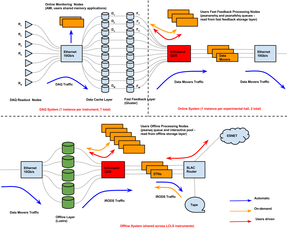
The following figure shows a logic diagram of the LCLS data flow and indicates the different stages where data analysis can be performed in LCLS: 

1. Online monitoring nodes - These nodes get the detector data over the network by snooping the multicast traffic between the DAQ readout nodes and the data cache layer. There is a set of monitoring nodes allocated for each instrument.
2. Fast feedback nodes - These nodes read the detector data from disk. It's possible to read the data quasi real time as they are written to the fast feedback (FFB) storage layer by the DAQ without the need to wait for the run to end. There is a farm of FFB nodes for each experimental hall.
3. Offline nodes - These nodes read the detector data from disk. These nodes, made of both interactive nodes (psana pool) and batch farms (psanaq queue, see below), are the main resource for doing data analysis and are shared across all LCLS instruments.
   
   

Image Added

Interactive Pool

In order to get access to the interactive nodes, connect to to psana:

ssh psana

The The psana pool is currently made of 5 servers with the following specifications:

...

LCLS provides a few Matlab licenses and one IDL license. Instructions on how to use these tools are in the the Matlab and  and IDL pages.

Two of the psana interactive nodes (psanagpu101 and 102) have GPUs. The other three (psanaphi101, 102 and 103) have Xeon Phi coprocessors.

...

There are a number of batch farms (i.e. collections  collections of compute nodes) located in the central computing building and in the NEH and FEH experimental halls. Instructions describing how to submit jobs can be found on the the Submitting Batch Job page page.

The main batch farm currently consist of 80 nodes with the following general specifications:

...

When performing analysis on the psana interactive nodes, it is is useful to display plots on your host machine. For host machines near SLAC, using ssh with X-windows forwarding (the -X or -Y options) suffices. X  windows forwarding can get slow for host machines in Europe. Some users have found better performance with technology called nomachine, this is documented on the Remote Visualization page page.

Prompt Analysis

There are various ways to get real time information about the data acquired by an LCLS experiment. Users should be aware of the different possibilities and choose the approach that works best for their experiment. The methods for doing prompt analysis are described here.

Resources

The following diagram shows a logic diagram of the LCLS data flow and indicates the different stages where data analysis can be performed in LCLS: 

1. Online monitoring nodes - These nodes get the detector data over the network by snooping the multicast traffic between the DAQ readout nodes and the data cache layer. There is a set of monitoring nodes allocated for each instrument.
2. Fast feedback nodes - These nodes read the detector data from disk. By using the live option in psana, it's possible to read the data quasi real time as they are written to the FFB storage layer by the DAQ without the need to wait for the run to end. There is a farm of FFB nodes for each experimental hall.
3. Offline nodes - These nodes read the detector data from disk. These nodes, made of both interactive nodes (psana pool) and batch farms (psanaq queue), are the main resource for doing data analysis and are shared across all LCLS instruments.

Image Removed

 described here.