Content
Experiment
COLTRIMS (Cold Target Recoil Ion Momentum Spectroscopy)
Data
on 2019-06-25 runs 91, 92, 93, 100 requested to restore from tape
/reg/d/psdm/AMO/amox27716/xtc/
exp=amox27716:run=100
event_keys -d exp=amox27716:run=100
Scripts and files
For exp=amox27716:run=100 in LCLS1 environment
- hexanode/examples/ex-quad-00-data.py - simple psana access to data and draws waveforms overlayed on the same plot
- hexanode/examples/ex-quad-01-cfd.py <Acqiris-chanel-number> - test of CFD (Constant Fraction Discriminator) parameters
- hexanode/examples/ex-quad-02-amox27716-0100-acqiris.py - advanced test of CFD with event loop and graphics
- hexanode/examples/ex-quad-07-proc-data-save-h5.py - processes waveforms in dataset and saves results for peaks in file like amox27716-r0100-e060000-single-node.h5
- hexanode/examples/ex-quad-09-sort-graph-data.py
- uses processed data from amox27716-r0100-e060000-single-node.h5 or raw (slow) exp=amox27716:run=100 and calibration files- /reg/d/psdm/amo/amox27716/calib/Acqiris::CalibV1/AmoEndstation.0:Acqiris.1/hex_config/0-end.dat - control anf config file
copy of /reg/d/psdm/xpp/xpptut15/calib/Acqiris::CalibV1/AmoETOF.0:Acqiris.0/hex_config/0-end.data - /reg/d/psdm/amo/amox27716/calib/Acqiris::CalibV1/AmoEndstation.0:Acqiris.1/hex_table/100-end.dat - table with results of the detector calibration
- /reg/d/psdm/amo/amox27716/calib/Acqiris::CalibV1/AmoEndstation.0:Acqiris.1/hex_config/0-end.dat - control anf config file
- hexanode/examples/ex-quad-10-sort-data.py - TBD
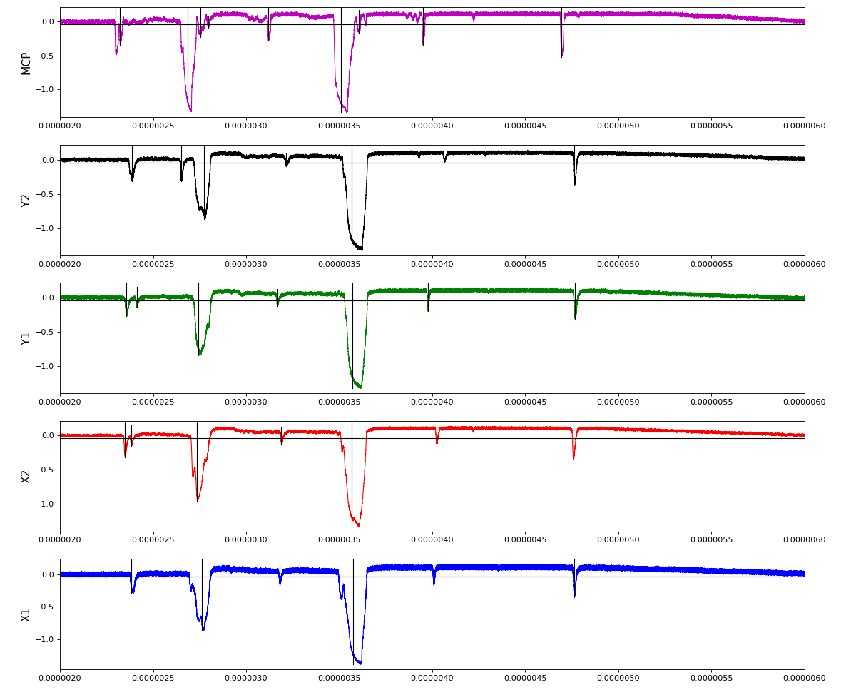
Waveforms
hex/examples/ex_acqiris_quad_amox27716-0100.py
Association of channels of AmoEndstation.0:Acqiris.1
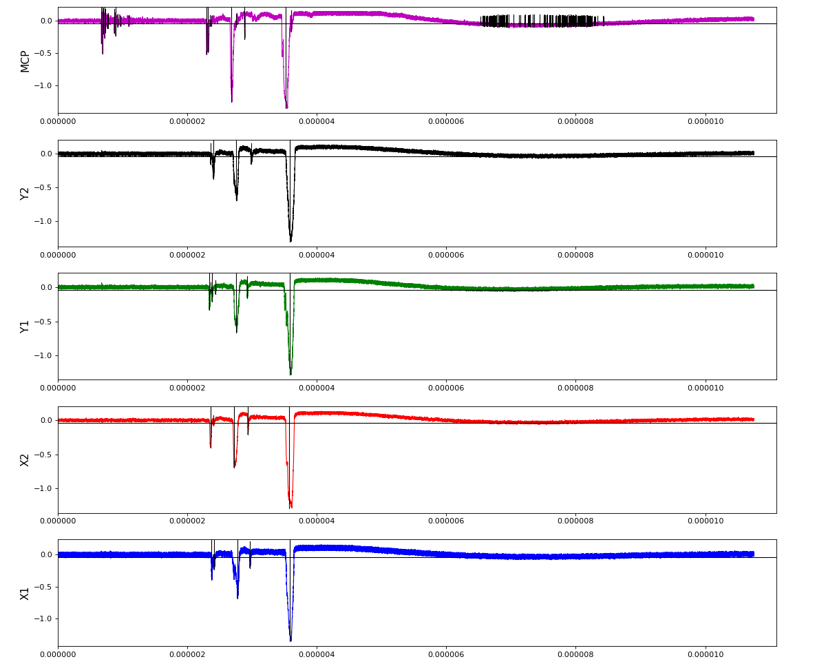
ch = (2,3,4,5,6) - all other channels of Acqiris.1 and 2 are empty or noisy
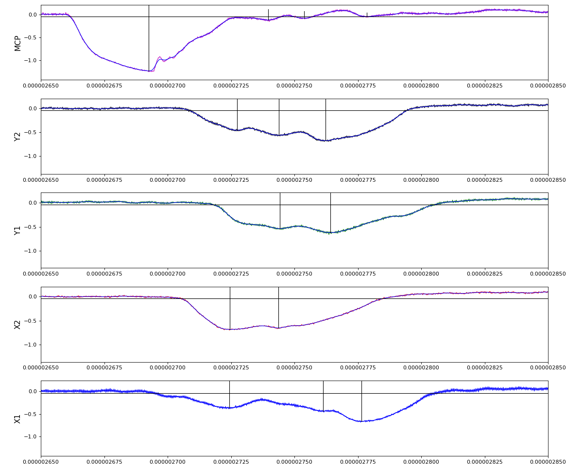
ylab = ('X1', 'X2', 'Y1', 'Y2', 'MCP')
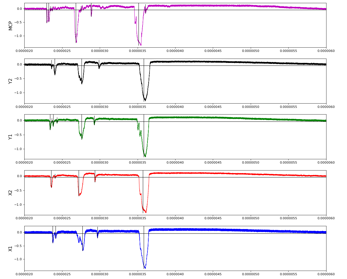
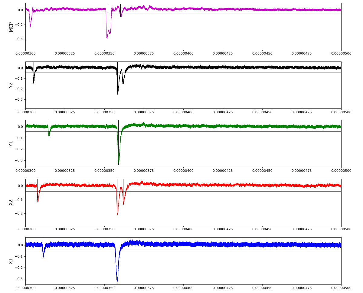
Other run amox27716 run 91 with lower hit density
Data processing
- hexanode/examples/ex-quad-02-amox27716-0100-acqiris.py - play with waveform parameters and the part of waveform WITHOUT NOISE!
- hexanode/examples/ex-quad-07-proc-data-save-h5.py - set w-f selection parameters data, detector channels, run over data and create hdf5 file.
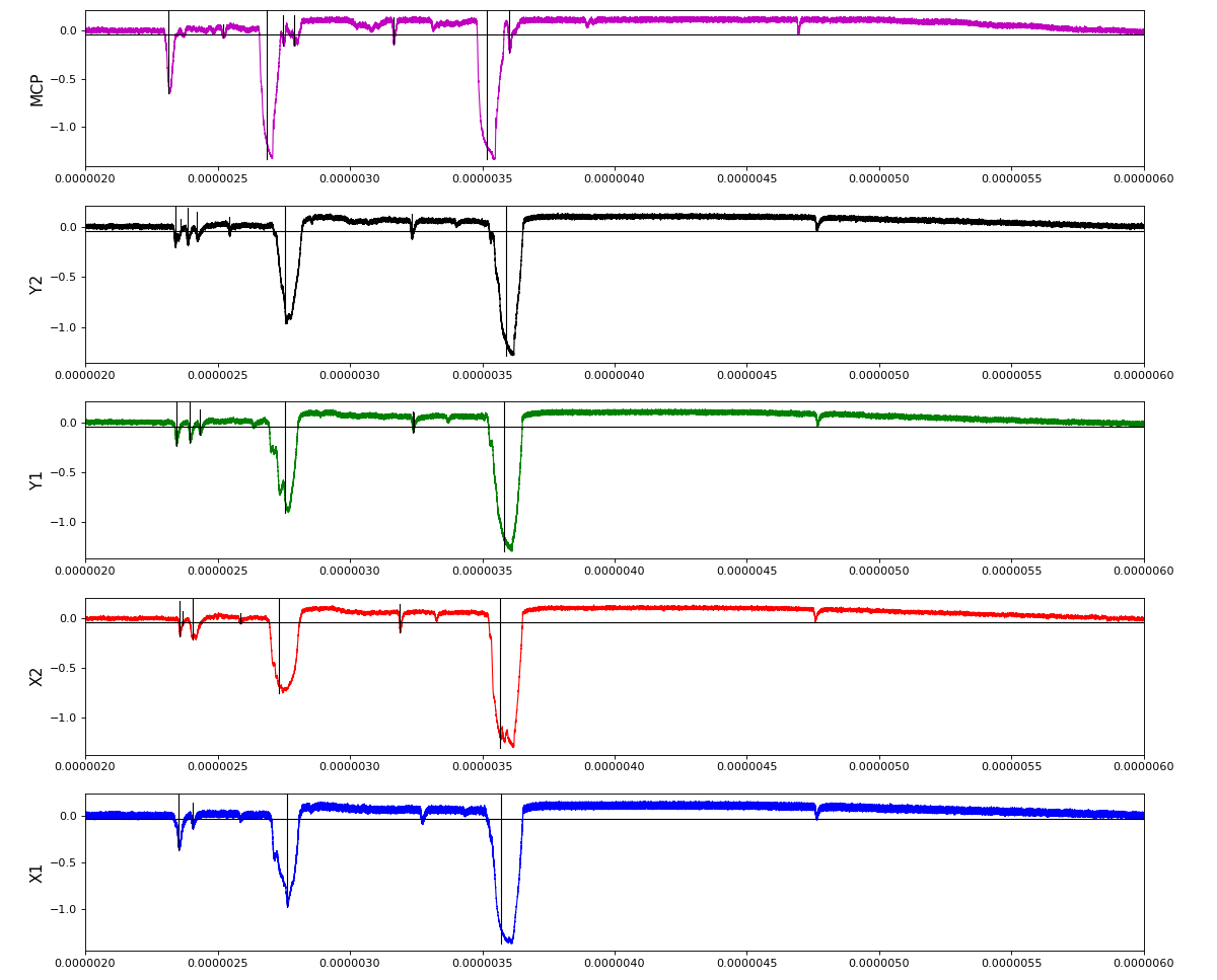
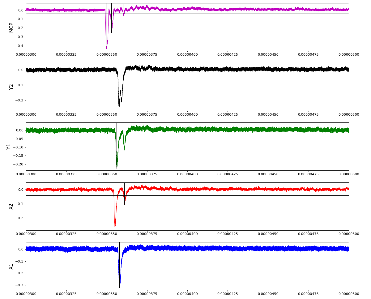
Total waveform with problematic peak reconstruction in MCP channel:
Test of local extreme peak-finder
Version of peak finder searching for local extremes after filtering
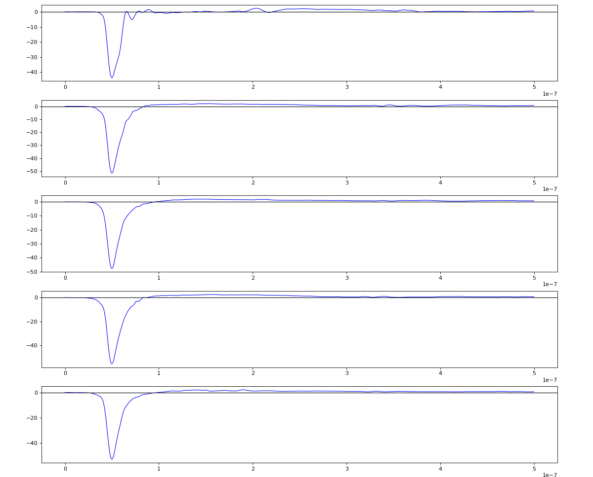
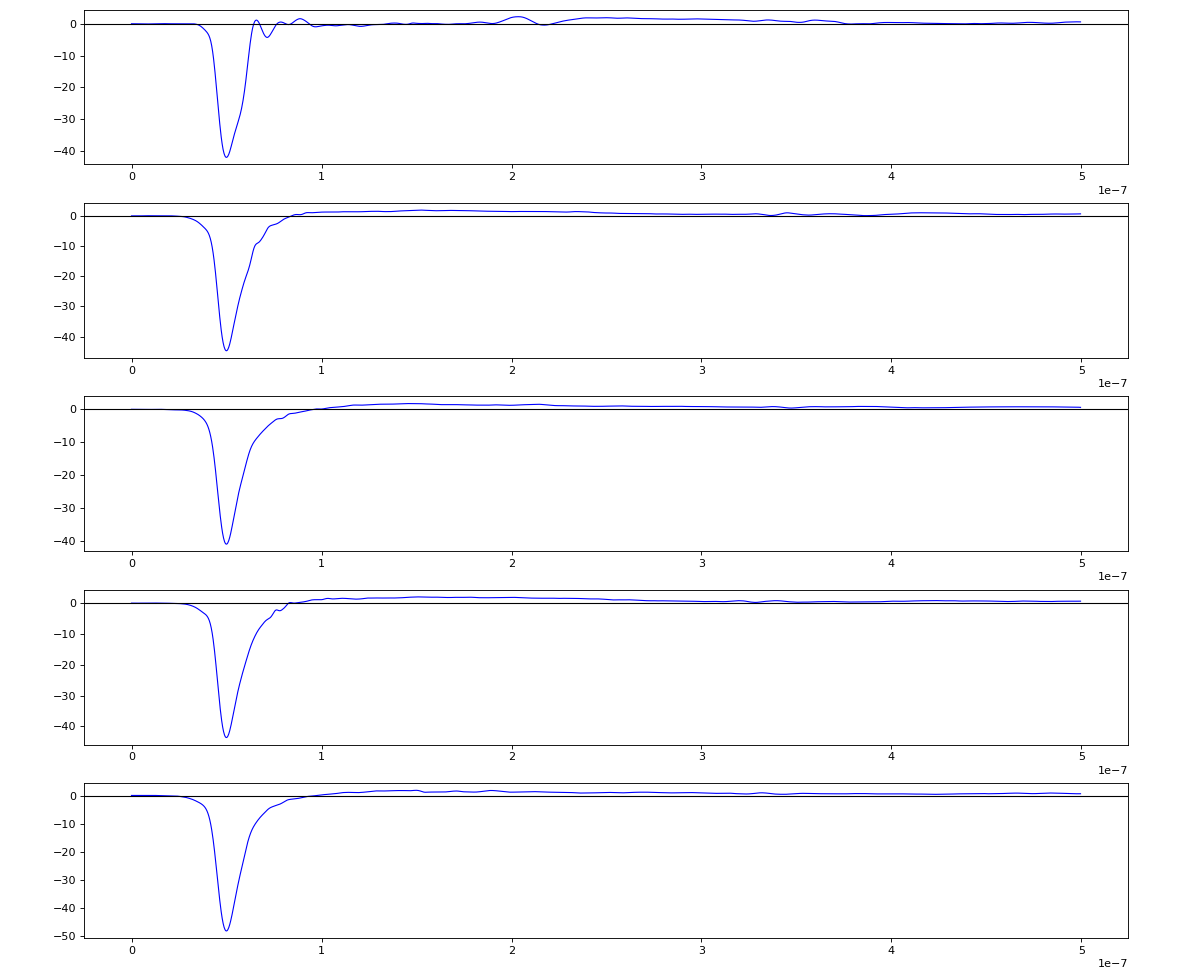
Wavelets estimation
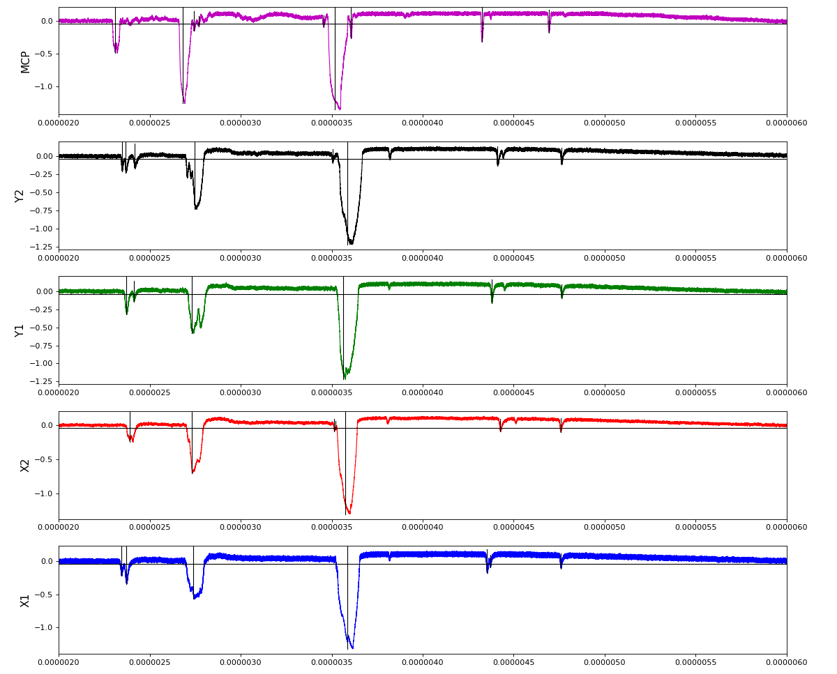
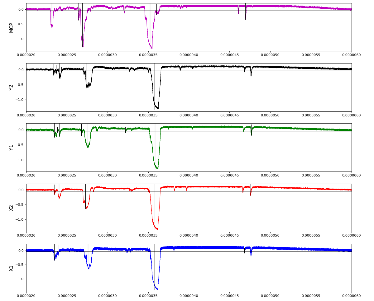
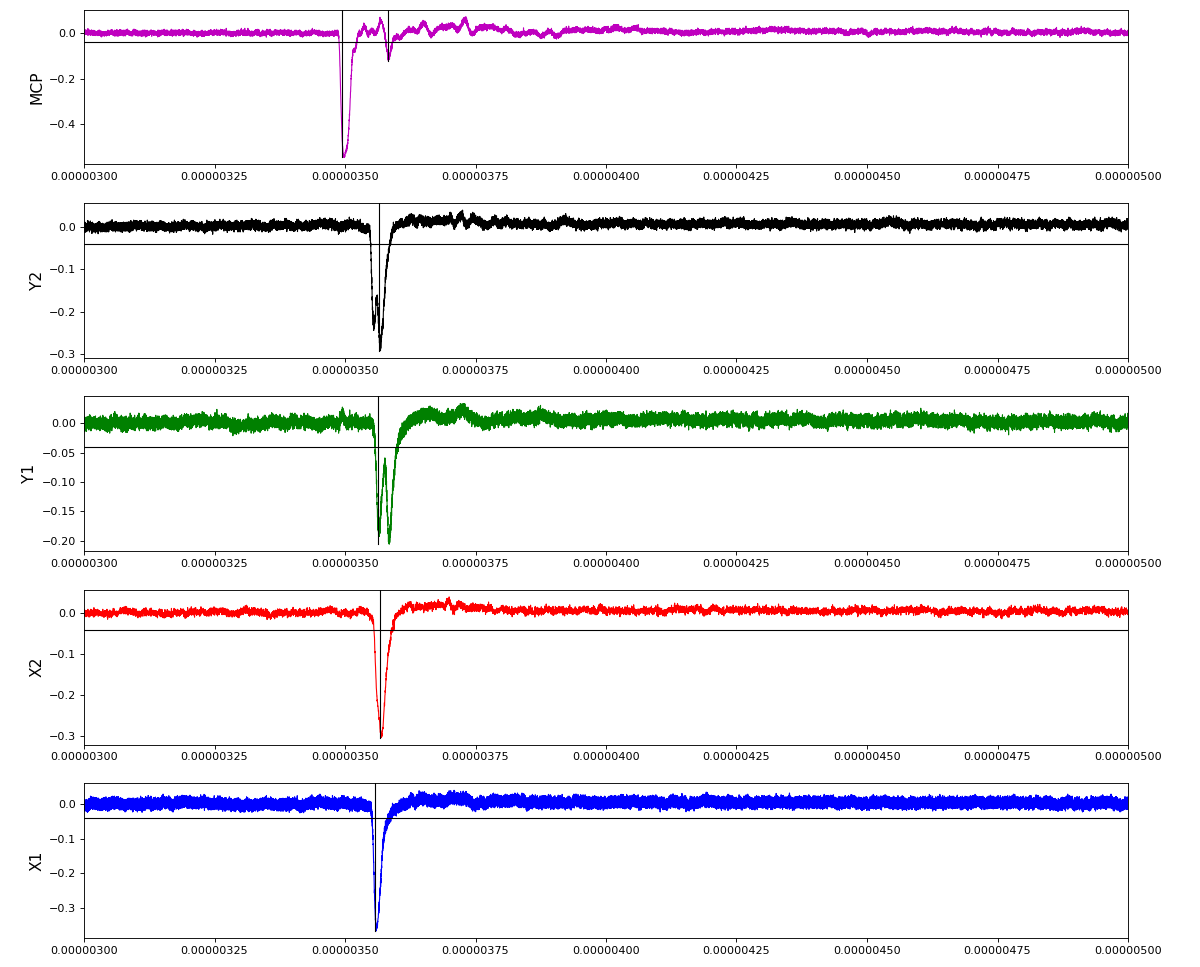
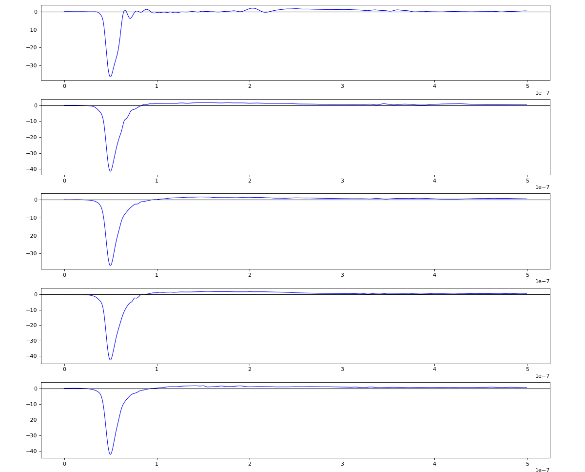
Waveform per channel averaged over 1k raw events with selection of a single peak for amox27716 runs 91,92, and 93
Calibration
Updated on 2020-10-08
Current hex-/quad-anode calibration procedure is not automated, and needs in expert manual operations...
Example scripts
- example scripts reside in the directory
lcls2/psana/psana/hexanode/examples/ - calibration of quad-anode requires two passes over ~105 events data set. There are two different approaches for calibration;
- slow calibration - run script like
ex-24-quad-proc-sort-graph.pytwo times directly on xtc2 data file for waveform processing and calibration. - faster calibration (x2 faster, especially helpful at development) - run script like
ex-22-data-acqiris-peaks-save-h5.pyorex-22-data-acqiris-peaks-save-h5-xiangli.pyonce on xtc2 data file for waveform processing and save intermediate results for number of hits per channel and times per channel in compact hdf5 file.- run script like
ex-23-quad-proc-sort-graph-from-h5.pytwo times on hdf5 data file for calibration.
- run script like
- slow calibration - run script like
- Approach 2 is used for further example because compact hdf5 file with 60k events is available in
/reg/g/psdm/detector/data_test/hdf5/amox27716-r0100-e060000-single-node.h5, but real xtc2 data files are not available yet.
What needs to be done in two calibration passes
Calibration pass 1
- edit file copied from
hexanode/examples/configuration_quad.txt- set the 1-st parameter "command" to 2.
make sure that the beginning 10 lines of this script are consistent with what you are doing, e.g.
2	// -1 = detector does not exist, 0 = just read (no sort/calib), 1 = sort, 2 = calibrate fu,fv,fw, w_offset, 3 = generate correction tables and write them to disk

0	// hexanode used (yes = 1, no = 0)  				(Parameter 1101)
0	// 0 = common start, 1 = common stop (for TDC8HP and fADC always use 0)

1	// TDC channel for u1 (counting starts at 1)			(Parameter 1129)
2	// TDC channel for u2 (counting starts at 1)			(Parameter 1130)
3	// TDC channel for v1 (counting starts at 1)			(Parameter 1131)
4	// TDC channel for v2 (counting starts at 1)			(Parameter 1132)
0	// TDC channel for w1 (counting starts at 1)			(Parameter 1133) HEX ONLY
0	// TDC channel for w2 (counting starts at 1)			(Parameter 1134) HEX ONLY
5	// TDC channel for mcp(counting starts at 1)  (0 if not used)	(Parameter 1135)
- in the script like
ex-23-quad-proc-sort-graph-from-h5.pyset path to the fileconfiguration_quad.txte.g.' calibcfg' : '/reg/neh/home4/dubrovin/LCLS/con-lcls2/lcls2/psana/psana/hexanode/examples/configuration_quad.txt', - After event loop is completed, this script generates a lot of histograms (BTW output histograms are controlled by the kwargs dict, see ex-23*).
- Look at resulting histograms and edit
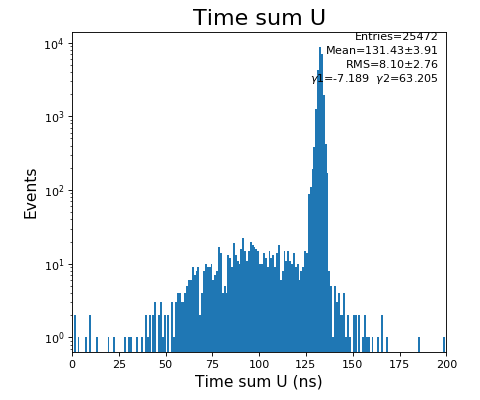
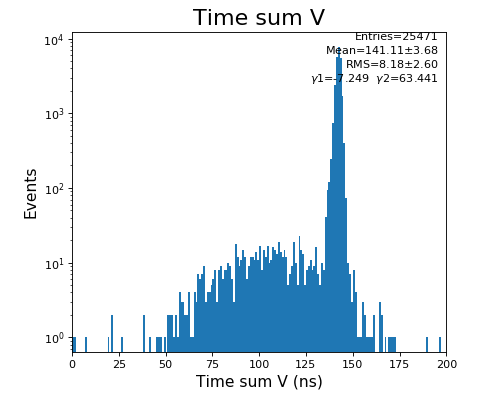
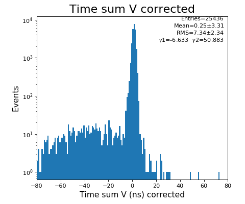
configuration_quad.txt- use Time sum U and V plots to set peak time value in Parameter 1108,1109
- then Halfwidth of the peak in this distribution to set Parameter 1115, 1116
- then Halfwidth of the u(ns), v(ns) distribution to set Parameter 1118, 1119
manually set scale-factor for layer U and V (mm/ns) Parameter 1102, 1103
Calibration parameters in the configuration_quad.txt-133.0 // offset to shift timesum layer U to zero (in nanoseconds) (Parameter 1108) -142.6 // offset to shift timesum layer V to zero (in nanoseconds) (Parameter 1109) 0 // offset to shift timesum layer W to zero (in nanoseconds) (Parameter 1110) HEX ONLY 0. // offset to shift the position picture in X (Parameter 1106) 0. // offset to shift the position picture in Y (Parameter 1107) 5.5 // halfwidth (at base) of timesum layer U (in nanoseconds) (Parameter 1115) 5.5 // halfwidth (at base) of timesum layer V (in nanoseconds) (Parameter 1116) 5.5 // halfwidth (at base) of timesum layer W (in nanoseconds) (Parameter 1117) HEX ONLY 1 // scalefactor for layer U (mm/ns) (Parameter 1102) 1 // scalefactor for layer V (mm/ns) (Parameter 1103) 1 // 0. scalefactor for layer W (Parameter 1104) HEX ONLY 1 // 0. offset layer W (in nanoseconds) (Parameter 1105) HEX ONLY 80. // runtime layer u (in nanosecods) (Parameter 1118) 80. // runtime layer v (in nanosecods) 0 means: same as u (Parameter 1119) 0. // runtime layer w (in nanosecods) 0 means: same as u (Parameter 1120) 40. // radius of active MCP area (in millimeters) (Parameter 1111)(always a bit larger than the real radius) 20. // deadtime of signals from the anode (Parameter 1121) 20. // deadtime of signals from the mcp (Parameter 1122) 1 // use position dependend correction of time sums? 0=no 1=yes (Parameter 1124) 0 // use position dependend NL-correction of position? 0=no 1=yes (Parameter 1125) HEX ONLY
Calibration pass 2
edit file configuration_quad.txt and set the 1-st parameter "command" to 3.
edit script like ex-23-quad-proc-sort-graph-from-h5.py and set pass where time correction table will be saved, e.g. 'calibtab' : '/reg/neh/home4/dubrovin/LCLS/con-lcls2/lcls2/psana/psana/hexanode/examples/calibration_table_data_new.txt'
run again script ex-23-quad-proc-sort-graph-from-h5.py
check results in calibration_table_data_new.txt
Post calibration arrangements
edit file configuration_quad.txt
set the 1-st parameter "command" to 1.
set Parameter 1124 in configuration_quad.txt
Both, configuration and calibration files need to be saved in calibration DB for automated data processing. This operation needs in actual experiment and detector names, run, timestamp, etc. Preliminary deployment commands:
cdb add -e amox27716 -d tmo_quadanode -c calibcfg -r 100 -f configuration_quad.txt     -i txt -u dubrovin
cdb add -e amox27716 -d tmo_quadanode -c calibtab -r 100 -f calibration_table_data.txt -i txt -u dubrovin
Content of the DB can be explored with GUI started by command calibman.
Automated data processing
See examples ex-24* or ex-25*.
Plots
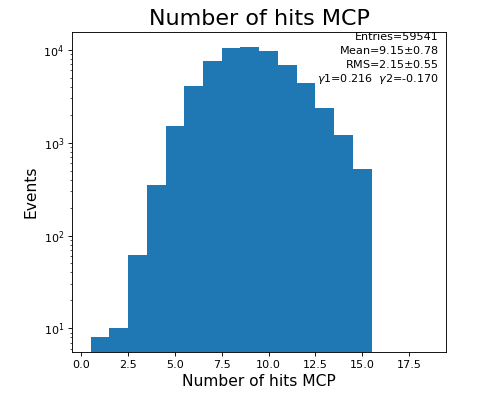
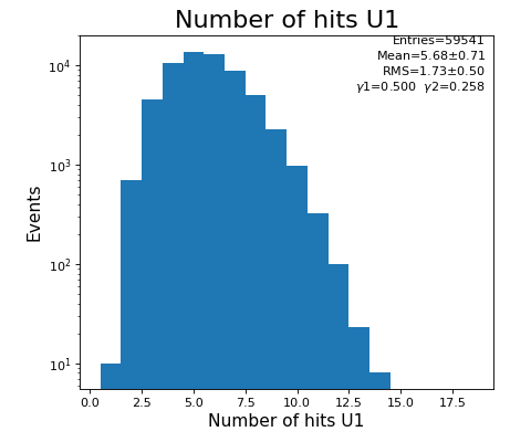
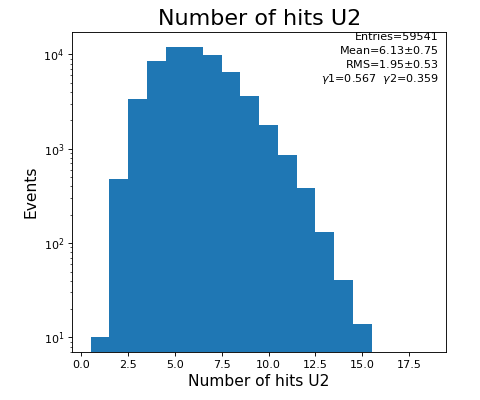
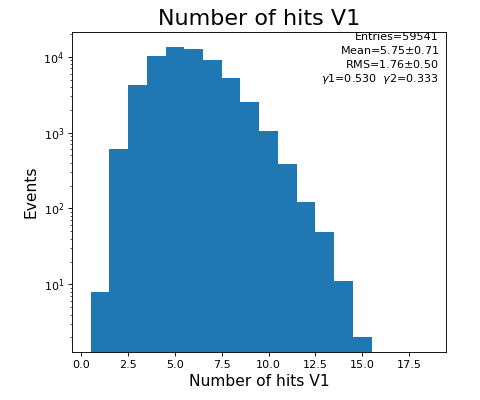
Number of hits per channel

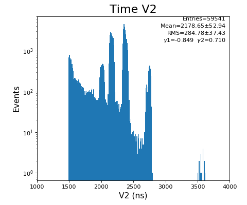
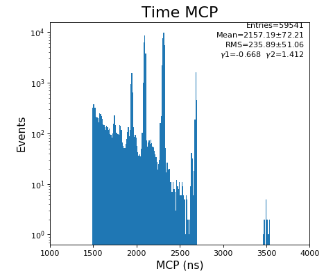
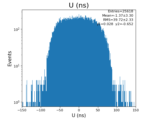
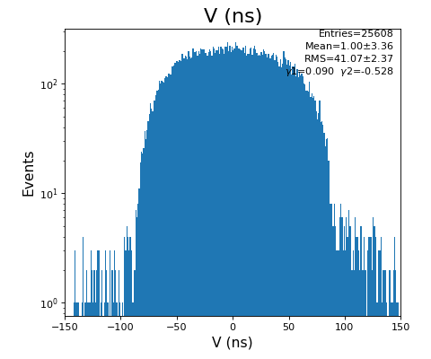
Spectra of time per channel, Spectra of U, V (ns)


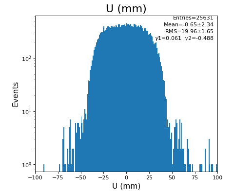
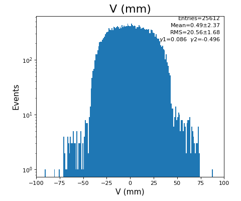
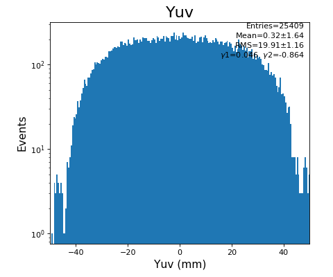
Spectra of U, V (mm)
Time sum (ns) for U, V
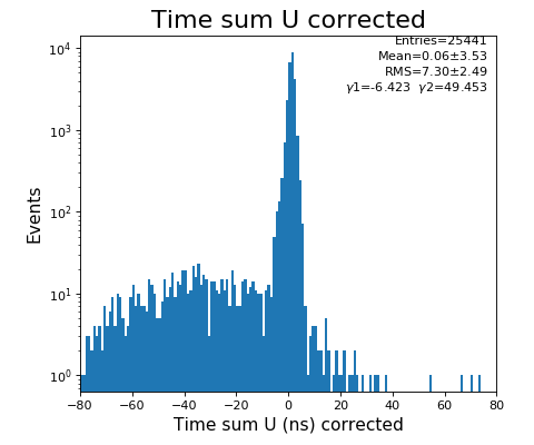
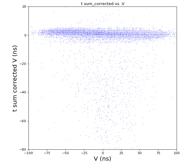
Time sum (ns) corrected for U, V
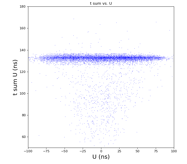
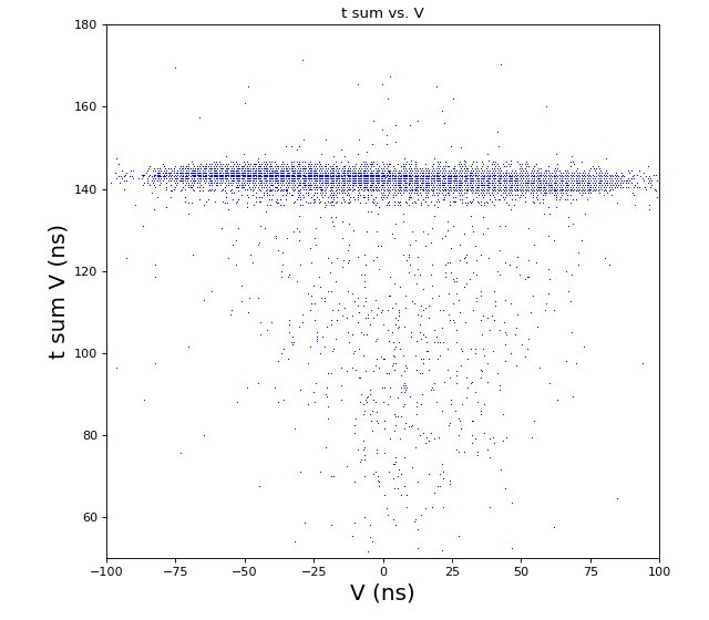
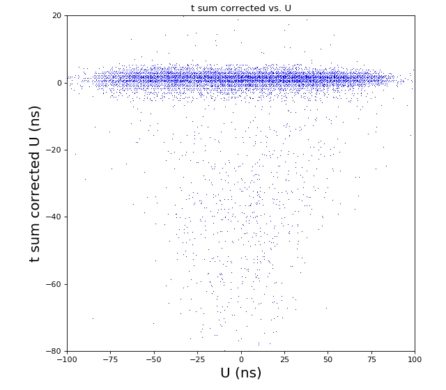
Time sum vs. variable U, V
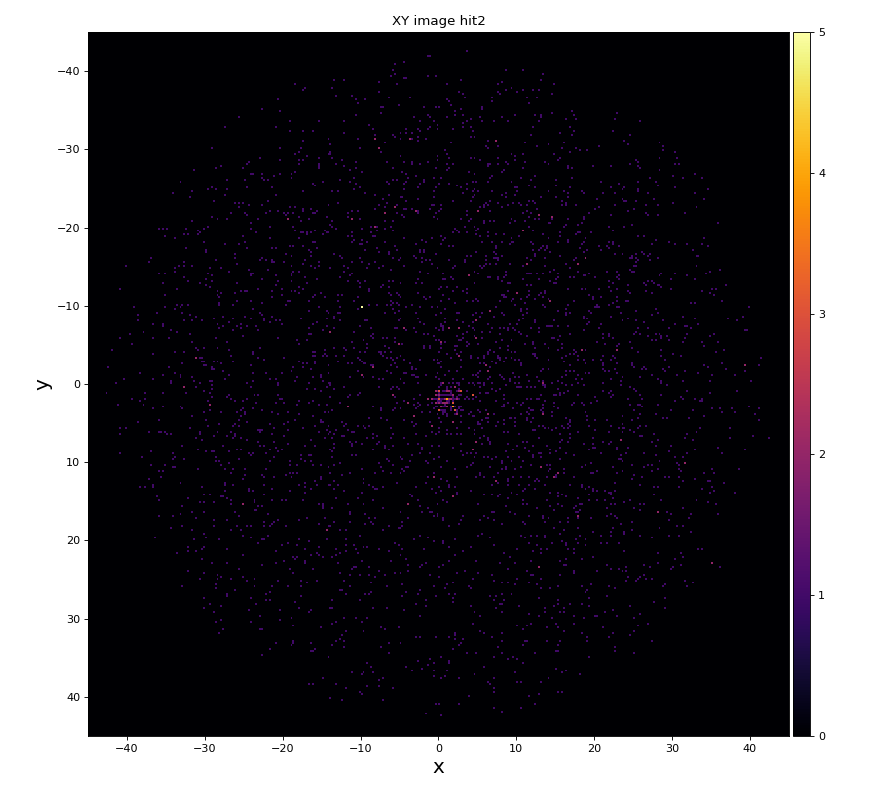
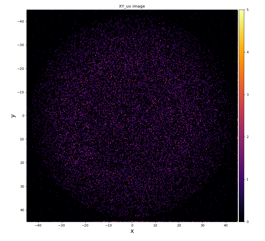
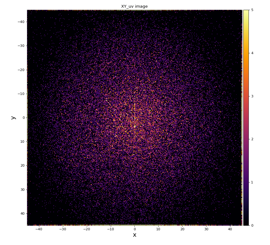
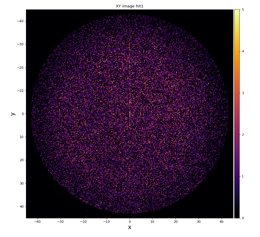
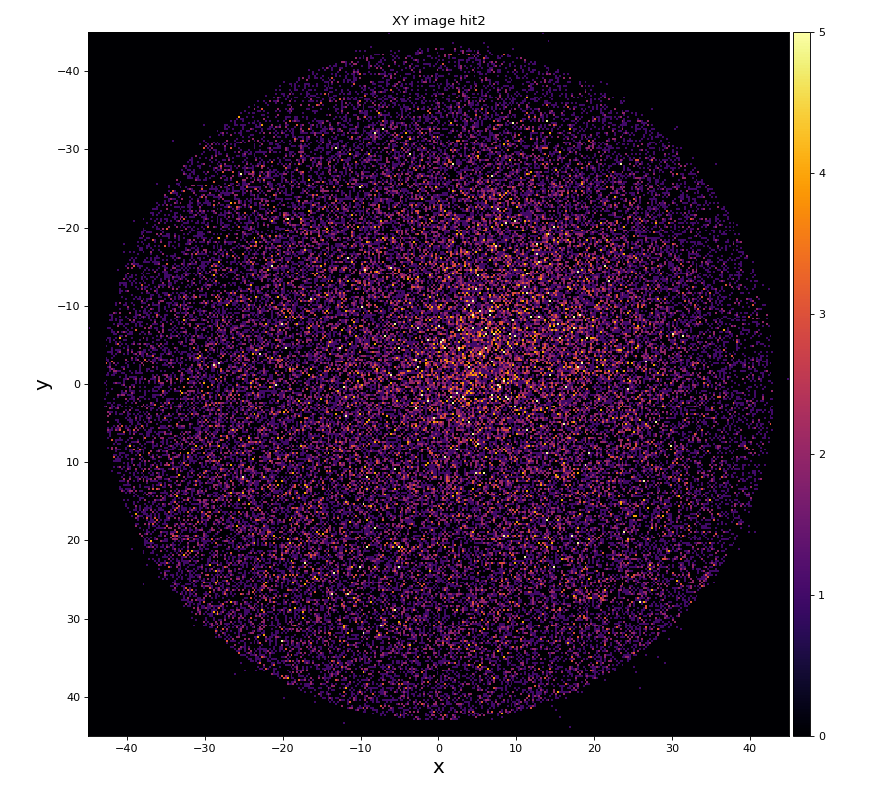
xy image for hit1 and 2

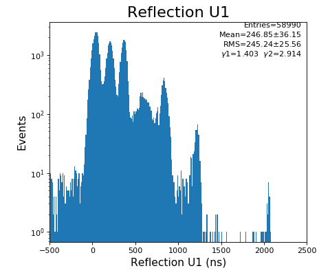
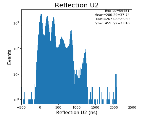
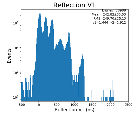
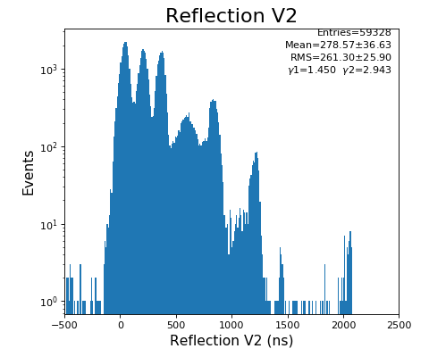
Reflection for all channels
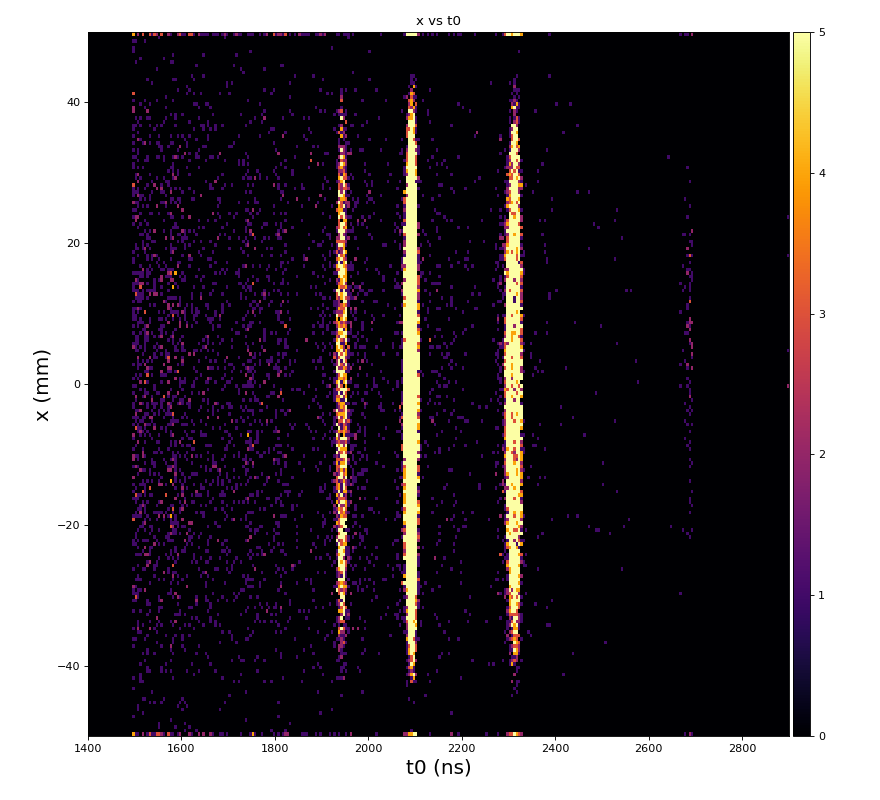
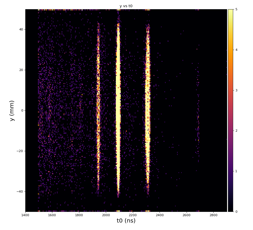
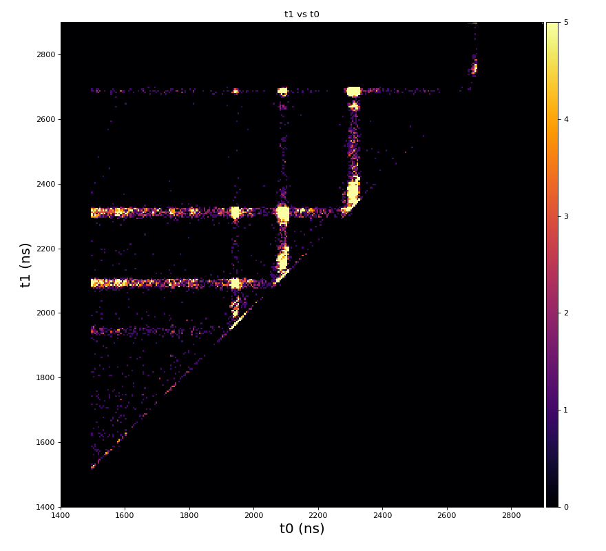
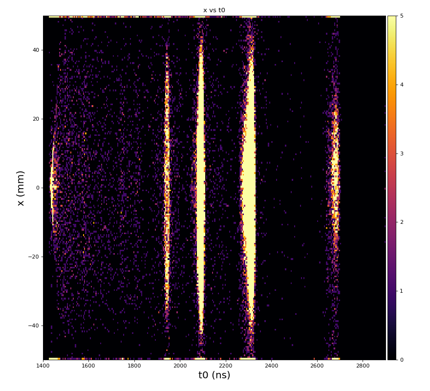
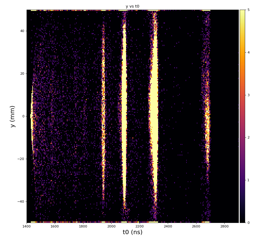
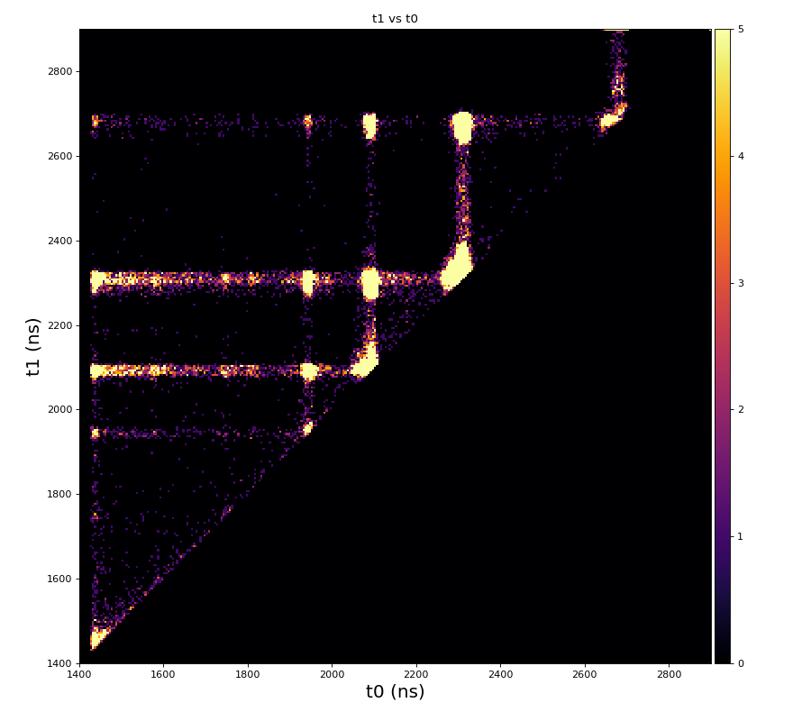
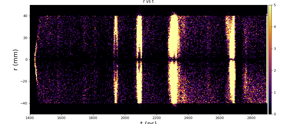
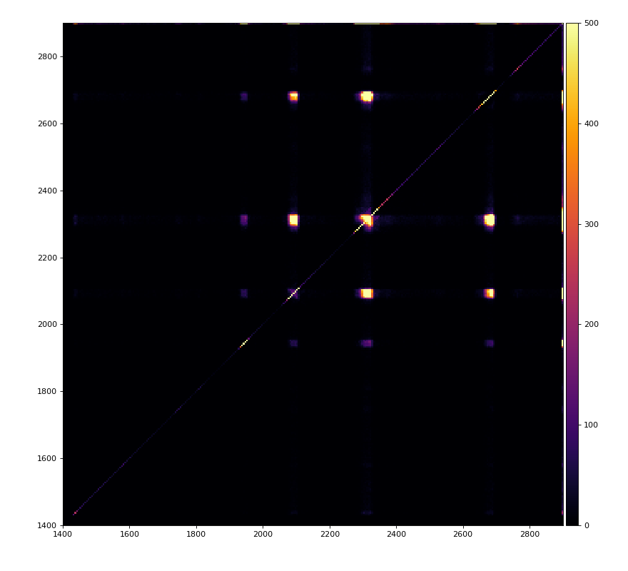
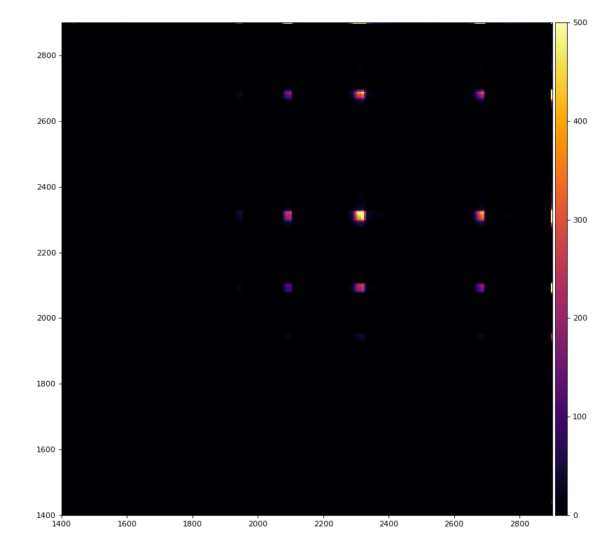
Physics plots t1,x,y vs t0
Calibrated plots
hexanode/examples/ex-quad-09-sort-graph-data.py with command 1 (after calibration command 2,3) set in configuration_quad.txt.
Soft on LCLS2
Examples
https://github.com/slac-lcls/lcls2/blob/master/psana/psana/hexanode/examples/
ex-20-data-acqiris-access.py - access to detector waveforms
ex-21-data-acqiris-graph.py - plot waveforms and found peaks
ex-22 - 24 - intended for calibration and representative graphics
ex-25-quad-proc-data.py - reads waveforms from xtc2, find peaks, and reconstruct hits using Roentdec library
Physics plots
From ex-23-quad-proc-sort-graph-from-h5.py or ex-24 if xtc2 file is available:
XTC2 trick
Only useful channels will be selected in xtc2. This hack is temporary available in
psana/psana/detector/test_detectors.py
Status on 2022-01-12
Project history
- This project was started with Timur Osipov in April 2015 in the framework of LCLS(1).
- RoentDec Co. commercially produces hex-/quad-anode cameras. Achim Czasch in co-operation with Timur has developed C++ library to process waveforms and sort signals from MCP with 2-/3-delay lines to reconstruct hits.
- Library is supplied in form of built module, without code to hide "secret" hit sorting algorithm.
- My job was to adopt this C++ library in our python algorithms.
- cython interface was developed to access in python major classes/methods of this c++ library.
- In the frame of this project unique development was done in the waveform analysis for peak finding; CWT/DWT - Current/Discrete Waveform Transformation, wavelet decomposition, BPF-Band Path Filter. This project was stopped as low-priority.
- In ~2019 RoentDec library and its pythonic interface were adopted in lcls2.
- ~2019 Xiang Li successfully replaced me in analysis business. Xiang brought his own CFD peak finder. I am still responsible for RoentDec library pythonic interface.
Recent development
Few days ago Chris asked me to check if RoentDec library interface still works. Due to relocation of different python and c++ modules in development of lcls2 software, compilation of examples for quad-anode was broken in ps-4.5.5/10. Now all visible issues are fixed and examples are working properly. Need in new release greater than ps-4.5.10.
List of test examples
Examples resides in lcls2/psana/psana/hexanode/examples/*
- ex-20-data-acqiris-access.py - access and print waveforms (times and intensities)
- ex-21-data-acqiris-graph.py - the same as ex-20 but with graphic plots
- ex-22-data-acqiris-peaks-save-h5.py - waveform processing by the (psana version of CFD) peakfinder and saving results in hdf5 file, 1000 events per 10 sec - 100Hz
- ex-22-data-acqiris-peaks-save-h5-xiangli.py - waveform processing by the (Xiang Li's version of CFD) peakfinder and saving results in hdf5 file, - 100Hz
- ex-23-quad-proc-sort-graph-from-h5.py - process peaks from hdf5 and apply RoentDec hit sorting algorithms, generate all signature-plots - 59999 events processing time = 104.848 sec or 0.001747 sec/event or 572.246 Hz
- ex-24-quad-proc-sort-graph.py - process peaks from xtc2 data and apply RoentDec hit sorting algorithms
- ex-25-quad-proc-data.py - similar to ex-24, demo how to get proc.xyrt_list
- ex-26-calibconsts.py - demo of access to calibration constants from DB
- ex-27-calib-pop-rbfs-xiang.py - demo of access to "rbfs" calibration constants from DB
Status on 2023-10-10
- Due to transition of software from psdm to s3df all ex-2*-* examples were updated
modified: ex-20-data-acqiris-access.py
modified: ex-21-data-acqiris-graph.py
modified: ex-22-data-acqiris-peaks-save-h5-xiangli.py
modified: ex-22-data-acqiris-peaks-save-h5.py
modified: ex-23-quad-proc-sort-graph-from-h5.py
modified: ex-24-quad-proc-sort-graph.py
modified: ex-25-quad-proc-data.py
modified: ex-26-calibconsts.py
modified: ex-27-calib-pop-rbfs-xiang.py
new file: ex_test_data.py
- File ex_test_data.py is added to define DIR_DATA_TEST depending on environment variable DIR_PSDM:
DIR_ROOT = os.getenv('DIR_PSDM') # /cds/group/psdm ON psana OR /sdf/group/lcls/ds/ana/ ON s3df
DIR_DATA_TEST = os.path.join(DIR_ROOT, 'detector/data2_test/xtc')
Then access to *.xtc2 files:
FNAME = '%s/%s' % (DIR_DATA_TEST, 'data-amox27716-r0100-acqiris-e000100.xtc2')
- Also changed access to the files in the package:
DIR_ABSPATH = os.path.abspath(os.path.dirname(__file__)) # absolute path to .../psana/hexanode/examples
+ 'calibcfg' : '%s/configuration_quad.txt' % DIR_ABSPATH,
+ 'calibtab' : '%s/calibration_table_data.txt' % DIR_ABSPATH,
All test examples are working.
References
Hexanode detector test on data
2019-11-01-Peter-Walter-article.pdf
Overview
Content Tools