- Flux, energy flux, and upper limit calculations for diffuse sources (22 Feb 2009)
- Diffuse response calculations and FITS image templates (22 Feb 2009)
- Analysis object creation using the hoops/ape interface
- Photon and Energy Flux Calculations
Flux, energy flux, and upper limit calculations for diffuse sources (22 Feb 2009)
pyLikelihood v1r10p1; Likelihood v14r4
Flux, energy flux and upper limit calculations can now be made for diffuse sources in the python interface:
>>> like.model
Extragalactic Diffuse
   Spectrum: PowerLaw
0      Prefactor:  1.450e+00  4.286e-01  1.000e-05  1.000e+02 ( 1.000e-07)
1          Index: -2.054e+00  1.366e-01 -3.500e+00 -1.000e+00 ( 1.000e+00)
2          Scale:  1.000e+02  0.000e+00  5.000e+01  2.000e+02 ( 1.000e+00) fixed

SNR_map
   Spectrum: PowerLaw2
3       Integral:  6.953e+03  2.566e+03  0.000e+00  1.000e+10 ( 1.000e-06)
4          Index: -2.039e+00  1.332e-01 -5.000e+00 -1.000e+00 ( 1.000e+00)
5     LowerLimit:  2.000e+01  0.000e+00  2.000e+01  2.000e+05 ( 1.000e+00) fixed
6     UpperLimit:  5.000e+05  0.000e+00  2.000e+01  5.000e+05 ( 1.000e+00) fixed

>>> like.flux('Extragalactic Diffuse', 100, 5e5)
0.00017279621316112551

>>> like.fluxError('Extragalactic Diffuse', 100, 5e5)
3.32420171199e-05

>>> like.flux('SNR_map', 100, 5e5)
1.3482399819603797e-06

>>> like.fluxError('W44_map', 100, 5e5)
2.54429802134e-07

>>> from UpperLimits import UpperLimits
>>> ul = UpperLimits(like)
>>> ul['Extragalactic Diffuse'].compute()
0 1.44990964752 0.000405768508472 0.000172805047298
1 1.62134142735 0.073917905358 0.000185125831974
2 1.79277320719 0.262761447131 0.000197078187151
3 1.96420498702 0.53963174062 0.00020864241284
4 2.13563676685 0.882155849953 0.000219869719057
5 2.33677514646 1.33948412506 0.000232753706737
6 2.37253076663 1.42681888532 0.000234966127989
(0.00023314676502589186, 2.34312748234)

>>> ul['SNR_map'].compute()
0 6953.47703963 7.03513949247e-05 1.34891151045e-06
1 7979.85337599 0.072031366891 1.43605234286e-06
2 9006.22971235 0.246899738264 1.51625454475e-06
3 10032.6060487 0.487519676687 1.59037705975e-06
4 11058.9823851 0.770755618154 1.65973696844e-06
5 12629.8902716 1.25421175769 1.75816622567e-06
6 13039.134979 1.38671547284 1.77783091654e-06
(1.7731240676197149e-06, 12941.1800697)
The values that are returned are the total fluxes for each source, i.e., integrated over all angles.
Diffuse response calculations and FITS image templates (22 Feb 2009)
Prior to Likelihood v14r3, there had been a long-standing problem with computing diffuse responses (with gtdiffrsp) for diffuse sources that have FITS image templates for discrete sources, such as SNRs or molecular clouds. In summary, gtdiffrsp performs the following integral for each diffuse source component
i
in the xml model definition:
\newcommand
\varepsilon
\newcommand
\varepsilon^\prime
\newcommand
{{\hat
}}
\newcommand
{{\hat
^\prime}}
\begin
\int d\phat S_i(\phat, \ep_j) A(\ep_j, \phat) P(\phatp_j; \ep_j, \phatp)
\end
where
$\hat
_j$
and
$\varepsilon^\prime_j$
are the measured direction and measured energy of detected photon
$j$
, and the integral is performed over (true) directions on the sky
$\hat
$
.
$A(...)$
and
$P(...)$
are the effective area and point spread function, and I have made the approximation equating the true photon energy with the measured value,
$\varepsilon = \varepsilon^\prime$
.
The problem arises for a discrete diffuse source when its spatial distribution
$S_i(\hat
)$
is only significantly different from zero far from the location of event
$j$
. Operationally, the integral is evaluated using an adaptive Romberg integrator that samples the integrand at theta and phi values that are referenced to
$\hat
_j$
. For very compact sources, the integrator will often miss the source entirely and evaluate the integral to zero, and unless the measured photon direction lies directly on the brightest part of the extended, the integral will usually not be very accurate, even if non-zero.
In Likelihood v14r3, the code has been modified to restrict the range of theta and phi values over which the integration is performed based on the boundaries of the input map. As long as the input map is not mostly filled with zero or near zero-valued entries, restricting the angular range this way seems to produce accurate diffuse response values.
This means that care should be made in preparing the FITS image templates used for defining diffuse sources in Likelihood. The map should be as small as possible and should exclude regions where the emission is negligible. Here are examples of bad (left) and good (right) template files for the same source:
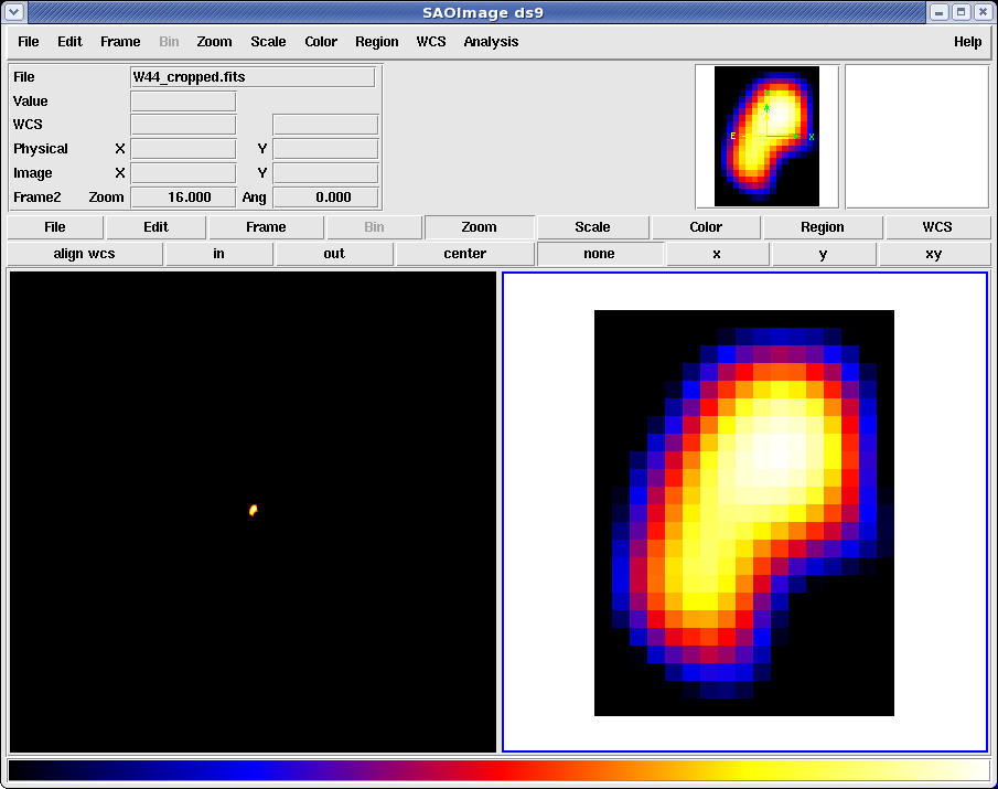
The FITS file on the left is 1000x1000 pixels most of which are zero. This is almost optimally bad. Except for events lying right on the source, the diffuse response integrals are almost all zero. The image on the right is the same data, but cropped to the 17x23 pixel region that actually contains relevant data. Performing an unbinned likelihood fit using this smaller map produces accurate results even in the presence of significant Galactic diffuse emission.
Analysis object creation using the hoops/ape interface
The UnbinnedAnalysis and BinnedAnalysis modules contain functions that use the hoops/pil/ape interface to take advantage of the gtlike.par file for specifying inputs. Usage of this interface may be more convenient than creating the UnbinnedObs, UnbinnedAnalysis, BinnedObs, and BinnedAnalysis objects directly. Here are some examples of their use:
- In this example, the call to the unbinnedAnalysis function is made without providing any arguments. The gtlike.par file is read from the user's PFILES path, and the various parameters are prompted for just as when running gtlike (except that the order is a bit different). If one is using the ipython interface with readline enabled, then tab-completion works as well.
>>> from UnbinnedAnalysis import *
>>> like = unbinnedAnalysis()
Response functions to use[P6_V1_DIFFUSE]
Spacecraft file[test_scData_0000.fits] test_scData_0000.fits
Event file[filtered.fits] filtered.fits
Unbinned exposure map[none]
Exposure hypercube file[expCube.fits]
Source model file[anticenter_model.xml]
Optimizer (DRMNFB|NEWMINUIT|MINUIT|DRMNGB|LBFGS) [MINUIT]
>>> like.model
Crab
   Spectrum: PowerLaw2
0       Integral:  1.540e+01  0.000e+00  1.000e-05  1.000e+03 ( 1.000e-06)
1          Index: -2.190e+00  0.000e+00 -5.000e+00  0.000e+00 ( 1.000e+00)
2     LowerLimit:  2.000e+01  0.000e+00  2.000e+01  3.000e+05 ( 1.000e+00) fixed
3     UpperLimit:  2.000e+05  0.000e+00  2.000e+01  3.000e+05 ( 1.000e+00) fixed

Geminga
   Spectrum: PowerLaw2
4       Integral:  1.020e+01  0.000e+00  1.000e-05  1.000e+03 ( 1.000e-06)
5          Index: -1.660e+00  0.000e+00 -5.000e+00  0.000e+00 ( 1.000e+00)
6     LowerLimit:  2.000e+01  0.000e+00  2.000e+01  3.000e+05 ( 1.000e+00) fixed
7     UpperLimit:  2.000e+05  0.000e+00  2.000e+01  3.000e+05 ( 1.000e+00) fixed

PKS 0528+134
   Spectrum: PowerLaw2
8       Integral:  9.802e+00  0.000e+00  1.000e-05  1.000e+03 ( 1.000e-06)
9          Index: -2.460e+00  0.000e+00 -5.000e+00  0.000e+00 ( 1.000e+00)
10    LowerLimit:  2.000e+01  0.000e+00  2.000e+01  3.000e+05 ( 1.000e+00) fixed
11    UpperLimit:  2.000e+05  0.000e+00  2.000e+01  3.000e+05 ( 1.000e+00) fixed
- Alternatively, one can give all of the parameters explicitly. This is useful for running in scripts.
>>> like2 = unbinnedAnalysis(evfile='filtered.fits', scfile='test_scData_0000.fits', irfs='P6_V1_DIFFUSE', expcube='expCube.fits', srcmdl='anticenter_model.xml', optimizer='minuit', expmap='none')
- The mode='h' option is available as well. In this case, one can set a specific parameter, leaving the remaining ones to be read silently from the gtlike.par file.
>>> like3 = unbinnedAnalysis(evfile='filtered.fits', mode='h')
- A BinnedAnalysis object may be created in a similar fashion using the binnedAnalysis function:
>>> from BinnedAnalysis import *
>>> like = binnedAnalysis()
Response functions to use[P6_V1_DIFFUSE::FRONT]
Counts map file[smaps_0_20_inc_front.fits]
Binned exposure map[binned_expmap_0_20_inc_front.fits]
Exposure hypercube file[expCube_0_20_inc.fits]
Source model file[Vela_model_0_20_inc_front.xml]
Optimizer (DRMNFB|NEWMINUIT|MINUIT|DRMNGB|LBFGS) [MINUIT]
Photon and Energy Flux Calculations
With Likelihood v13r18 and pyLikelihood v1r6 (ST v9r8), a facility has been added for calculating photon (ph/cm^2/s) and energy (MeV/cm^2/s) fluxes over a selectable energy range. The errors on these quantities are computed using the procedure described in this presentation made at the [September 2008 Collaboration meeting]. Here are some usage examples:
>>> like.model
Extragalactic Diffuse
   Spectrum: PowerLaw
0      Prefactor:  7.527e-02  7.807e-01  1.000e-05  1.000e+02 ( 1.000e-07)
1          Index: -2.421e+00  1.968e+00 -3.500e+00 -1.000e+00 ( 1.000e+00)
2          Scale:  1.000e+02  0.000e+00  5.000e+01  2.000e+02 ( 1.000e+00) fixed

GalProp Diffuse
   Spectrum: ConstantValue
3          Value:  1.186e+00  5.273e-02  0.000e+00  1.000e+01 ( 1.000e+00)

Vela
   Spectrum: BrokenPowerLaw2
4       Integral:  9.176e-02  3.730e-03  1.000e-03  1.000e+03 ( 1.000e-04)
5         Index1: -1.683e+00  5.131e-02 -5.000e+00 -1.000e+00 ( 1.000e+00)
6         Index2: -3.077e+00  2.266e-01 -5.000e+00 -1.000e+00 ( 1.000e+00)
7     BreakValue:  1.716e+03  2.250e+02  3.000e+01  1.000e+04 ( 1.000e+00)
8     LowerLimit:  1.000e+02  0.000e+00  2.000e+01  2.000e+05 ( 1.000e+00) fixed
9     UpperLimit:  3.000e+05  0.000e+00  2.000e+01  5.000e+05 ( 1.000e+00) fixed

>>> like.flux('Vela', emin=100, emax=3e5)
9.2005203669330761e-06

>>> like.flux('Vela')
9.2005203669330761e-06

>>> like.fluxError('Vela')
3.73060211564e-07

>>> like.energyFlux('Vela')
0.0047870395747710718

>>> like.energyFluxError('Vela')
0.000260743911378
The default energy range for the flux and energy flux calculations is (emin, emax) = (100, 3e5) MeV. Either or both of these may be set as keyword arguments to the function call. The errors are available as separate function calls and require that the covariance matrix has been computed using "covar=True" keyword option to the fit function:
>>> like.fit(covar=True)