- Calculating SEDs directly from pyLikelihood (8 November 2011)
- Prior distributions on fit parameters (4 February 2011)
- User defined error and contour level in Minos (3 May 2010)
- Composite2 (11 July 2010)
- RadialProfile model (5 July 2010)
- gtsrcprob tool: Presentation to 14 May 2010 WAM (See also LK-57@JIRA.)
- Upper limits using the (semi-)Bayesian method of Helene (21 September 2009)
- Interface to MINOS errors from Minuit or NewMinuit (29 June 2009)
- EBL Attenuation models (20 June 2009)
- SummedLikelihood (11 June 2009)
- SmoothBrokenPowerLaw (11 June 2009)
- Flux, energy flux, and upper limit calculations for diffuse sources (22 Feb 2009)
- Diffuse response calculations and FITS image templates (22 Feb 2009)
- Analysis object creation using the hoops/ape interface
- Photon and Energy Flux Calculations
Calculating SEDs directly from pyLikelihood (8 November 2011)
SEDs can be computed directly from pyLikelihod using a new SED class.
This code has the advantage that it does not create any temporary files and does not require multiple gtlike jobs or xml files. The only additional dependency of the code is scipy.
Usage example:
# SEDs can only be computed for binned analysis.
# First, created the BinnedAnalysis object...
like=BinnedAnalysis(...)

...

# Now created the SED object

# This object is in pyLikelihood
from SED import SED

name='Vela'
sed = SED(like,name)

# There are many helpful flags to modify how the SED is created
sed = SED(like,name,
          # minimum TS in which to compute an upper limit
          min_ts=4,

          # Upper limit algoirthm: bayesian or frequentist
          ul_algorithm='bayesian',

          # confidence level of upper limtis
          ul_confidence=.95,

          # By default, the energy binning is consistent with
          # the binning in the ft1 file. This can be modified, but the
          # new bins must line up with the ft1 file's bin edges
          bin_edges = [1e2, 1e3, 1e4, 1e4])

# save data points to a file
sed.save('sed_Vela.dat')

# The SED can be plotted
sed.plot('sed_Vela.png')

# And finally, the results of the SED fit can be packaged
# into a convenient dictionary for further use

results=sed.todict()

# To load the data points into a new python script:
results_dictionary=eval(open('sed_vela.dat').read())
Prior distributions on fit parameters (4 February 2011)
optimizers-02-21-00, Likelihood-17-05-01, pyLikelihood-01-27-01
1D priors can now be assigned to individual fit parameters in the Python interface. The current implementation allows for Gaussian pdfs, but the interface can also accomodate other pdfs: the corresponding Function classes just need to be implemented.
Usage examples:
>>> like[i].addGaussianPrior(-2.3, 0.1)   # Add a Gaussian prior to parameter i with a mean value of -2.3 and root-variance (sigma) of 0.1

>>> like[i].addPrior('LogGaussian')       # Add a prior function by name.  Default parameter values will be used.

>>> print like[i].getPriorParams()        # This returns a dictionary of the parameters of the function representing the pdf.
{'Sigma': 0.01, 'Norm': 1.0, 'Mean':-2.29999999999999998}

>>> like[i].setGaussianPriorParams(-2.3, 0.01)    # Set the prior parameter values (mean, sigma) for the Gaussian case.

>>> like[i].setPriorParams(Mean=-2.3)      # Set the prior parameter values by name for any prior function.
User defined error and contour level in Minos (3 May 2010)
optimizers-02-18-00
In MINUIT parlance, the parameter UP defines the error level returned by the routines MIGRAD/HESSE/MINOS. If FCN is the function to be minimized, the returned error is this value which, added to the best fit value of the parameter, increases FCN by an amount of UP. If FCN is the usual chi-square function (a.k.a weighted least square function), UP=1 yields the usual 1-sigma error. If FCN is minus the log Likelihood function, then UP=0.5 yields the 1-sigma error. In the ScienceTools, the optimizers package defines the FCN as minus the log likelihood function. The new implementation allow the user to define the error level he wish to obtain from MINUIT, via the "level" argument, which is defined as : UP=level/2. It is the responsibility of the user to understand what "level" should be, depending on his use case. What the code implementation ensures is the following : "level" is that value of the function -2DeltaLogLikelihood(p) that, when reached for a parameter value p, will drive MINUIT to return as the error the value (p-p_min), where p_min is the best fit value of the parameter p. Under the assumption that -2DeltaLogLikelihood is distributed as the chi-square probability distribution with one degree of freedom, level=4 with thus yield two-sided 2-sigma errors. This is because there is 5% of the total chi2 density beyond the value 4 (actually ~3.85), which translates into 2-sigma errors, as there is 2.5% of the Normal probability density beyond 2 (actually ~2.3%), and we are looking at 2-sided confidence intervals.
Finally, the MNCONTOUR contour analysis from MINUIT, which essentially runs MINOS on a pair of parameters, is now also exposed. This needs further testing, and API improvement so that the resulting contour points can be returned within python : they are currently just printed out onscreen, together with the contour (ascii plotting like in the old days :) ). Take note that these are now 2-parameter errors, so that level=1 is not a 1-sigma contour (though you do get the 1-sigma one parameter errors by projecting the extrema of the contour along the corresponding axis).
For more information on MINUIT? please look at the original manual for the FORTRAN code , and the the C++ user's guide.
Composite2 (11 July 2010)
Likelihood-16-10-00, pyLikelihood-01-25-00
This is similar to the CompositeLikelihod and SummedLikelihood classes (all three are accessible via the pyLikelihood interface) in that log-likelihood objects may be combined to form a single objective function. Composite2 allows users to tie together arbitrary sets of parameter across (and within) the different log-likelihood components of the composite. It can therefore reproduce the functionality of the CompositeLikelihood model, where the parameters, except for the normalizations, for the "stacked" sources are tied together; it can also reproduce the functionality of the SummedLikelihood, where all of the corresponding parameters for models of the different components are tied together. The SummedLikelihood implementation is still preferred for that application since it supports the UpperLimits.py and IntegralUpperLimit.py modules whereas Composite2 does not. Composite2 does support the minosError function that is also available from CompositeLikelihood. Composite2 has not been extensively tested.
Here are scripts that demonstrate the Composite2 equivalence to CompositeLikelihood and SummedLikelihood. For clarity, here is the xml model file used with those scripts.
RadialProfile model (5 July 2010)
Likelihood-16-08-02
Similar to the RadialSource model in celestialSource/genericSources, this model defines an azimuthally symmetric diffuse source that is specified by an ascii file containing the radial profile as a function of off-source angle.
<source name="test_profile" type="DiffuseSource">
   <spectrum type="PowerLaw">
     <parameter free="1" max="1000.0" min="0.001" name="Prefactor" scale="1e-09" value="10.0"/>
     <parameter free="1" max="-1.0" min="-5.0" name="Index" scale="1.0" value="-2.0"/>
     <parameter free="0" max="2000.0" min="30.0" name="Scale" scale="1.0" value="100.0"/>
   </spectrum>
   <spatialModel type="RadialProfile" file="radial_profile.txt">
     <parameter free="0" max="10" min="0" name="Normalization" scale="1.0" value="1"/>
     <parameter free="0" max="360." min="-360" name="RA" scale="1.0" value="82.74"/>
     <parameter free="0" max="90" min="-90" name="DEC" scale="1.0" value="13.38"/>
   </spatialModel>
 </source>
An example template file for the radial profile is attached. The first column is the offset angle in degrees from the source center (given by RA, DEC in the xml model def), and the second column is the differential intensity. The units of the function in that file times the spectral part of the xml model definition should be photons/cm^2/s/sr, just as for any other diffuse source.
NB: Linear interpolation is used for evaluating the profile using the points in the template file, and the code will simply try to extrapolate beyond the first and last entries. So the first point should be at offset zero, and the last two entries should both be set to zero intensity, otherwise the extrapolation can go negative at large angles.
This source has not been extensively tested.
Upper limits using the (semi-)Bayesian method of Helene (21 September 2009)
pyLikelihood v1r17
For background, see Stephen Fegan's presentation to the Catalog group.
This functionality is now available in two ways: as a new method, bayesianUL(...), in the existing UpperLimit class, and as a separate function in the IntegralUpperLimit.py module. The latter was implemented by Stephen using scipy (which we do not distribute with ST python). The bayesianUL(...) method does not require scipy and can only be run after UpperLimit.compute(...) is run first. The scipy version is more robust in some cases; the bayesianUL(...) function can return a spuriously low upper limit if the pyLikelihood object is not initially at a good minimum.
Example of usage:
from UnbinnedAnalysis import *
import UpperLimits
import IntegralUpperLimit    # This requires scipy

like = unbinnedAnalysis(evfile='filtered.fits',
                        scfile='test_scData_0000.fits',
                        expmap='expMap.fits',
                        expcube='expCube.fits',
                        srcmdl='srcModel.xml',
                        irfs='P6_V3_DIFFUSE',
                        optimizer='MINUIT')

src = 'my_source'

emin = 100
emax = 3e5

PhIndex = like.par_index(src, 'Index')
like[PhIndex] = -2.2
like.freeze(PhIndex)

like.fit(0)

ul = UpperLimits.UpperLimits(like)
ul_prof, par_prof = ul[src].compute(emin=emin, emax=emax, delta=2.71/2)

print "Upper limit using profile method: ", ul_prof

ul_bayes, par_bayes = ul[src].bayesianUL(emin=emin, emax=emax, cl=0.95)

print "Using default implementation of method of Helene: ", ul_bayes

ul_scipy, results_scipy = IntegralUpperLimit.calc(like, src, ul=0.95,
                                                  emin=emin, emax=emax)

print "Using S. Fegan's module (requiring scipy): ", ul_scipy
Output (note use of the local ipython, which has scipy installed):
ki-rh2[jchiang] which ipython
/afs/slac/g/ki/software/python/2.5.1/i386_linux26/bin/ipython
ki-rh2[jchiang] ipython analysis.py
0 0.005535583927 2.21673610667e-06 8.05446445813e-07
1 0.00700983628826 0.0713089268528 1.01995522036e-06
2 0.00848408864951 0.24764020254 1.23446399491e-06
3 0.00995834101077 0.49775117816 1.44897276946e-06
4 0.011432593372 0.802803851635 1.66348154402e-06
5 0.0135311686428 1.30808036117 1.96883144303e-06
6 0.0139522586249 1.417706337 2.03010147956e-06
Upper limit using profile method:  1.99505486283e-06
Using default implementation of method of Helene:  2.29836280879e-06
Using S. Fegan's module (requiring scipy):  2.31242668344e-06
Python 2.5.1 (r251:54863, May 23 2007, 23:16:17)
Type "copyright", "credits" or "license" for more information.

IPython 0.8.1 -- An enhanced Interactive Python.
?       -> Introduction to IPython's features.
%magic  -> Information about IPython's 'magic' % functions.
help    -> Python's own help system.
object? -> Details about 'object'. ?object also works, ?? prints more.

In [1]:
As usual, the units of the flux upper limits are photons/cm^2/s.
Interface to MINOS errors from Minuit or NewMinuit (29 June 2009)
optimizers v2r17p1, pyLikelihood v1r15
The Minuit and Minuit2 (NewMinuit) libraries can calculate asymmetric errors that are based on the profile likelihood method. I've modified the python interface in pyLikelihood to make it easier to have the code evaluate these errors. Note that these errors are only available for the 'Minuit' and 'NewMinuit' optimizers.
Here is a script illustrating the interface. Parameters can be specified by index number (as displayed by "print like.model") or by source name and parameter name:
from UnbinnedAnalysis import *

like = unbinnedAnalysis(mode='h',
                        optimizer='NewMinuit',
                        evfile='ft1_03.fits',
                        scfile='FT2.fits',
                        srcmdl='3c273_03.xml',
                        expmap='expMap_03_P6_V3.fits',
                        expcube='expCube_03_P6_V3.fits',
                        irfs='P6_V3_DIFFUSE')

try:
    print like.minosError('3C 273', 'Integral')
except RuntimeError, message:
    print "Caught a RuntimeError: "
    print message

like.fit(0)

print like.model

print "Minos errors:"
print "3C 273, Integral: ", like.minosError('3C 273', 'Integral')
print "3C 273, Integral: ", like.minosError(0)
print "3C 273, Index: ", like.minosError('3C 273', 'Index')

try:
    print "ASO0267, Integral:", like.minosError('ASO0267', 'Integral')
except RuntimeError:
    par_index = like.par_index('ASO0267', 'Integral')
    print "ASO0267, Integral parameter index: ", par_index
    print "Parabolic error estimate: ", like[par_index].error()
The function 'like.par_index(...)' is also new. It returns the index of the parameter when given the source and parameter names.
Here is the output:
Caught a RuntimeError:
To evaluate minos errors, a fit must first be performed using the Minuit or NewMinuit optimizers.

<...skip some unsupressable Minuit2 output...>

3C 273
   Spectrum: PowerLaw2

0       Integral:  7.343e-01  2.525e-01  1.000e-05  1.000e+03 ( 1.000e-06)
1          Index: -2.592e+00  2.824e-01 -5.000e+00 -1.000e+00 ( 1.000e+00)
2     LowerLimit:  1.000e+02  0.000e+00  2.000e+01  2.000e+05 ( 1.000e+00) fixed
3     UpperLimit:  3.000e+05  0.000e+00  2.000e+01  3.000e+05 ( 1.000e+00) fixed

3C 279
   Spectrum: PowerLaw2
4       Integral:  1.241e+00  4.307e-01  1.000e-05  1.000e+03 ( 1.000e-06)
5          Index: -2.981e+00  3.197e-01 -5.000e+00 -1.000e+00 ( 1.000e+00)
6     LowerLimit:  1.000e+02  0.000e+00  2.000e+01  2.000e+05 ( 1.000e+00) fixed
7     UpperLimit:  3.000e+05  0.000e+00  2.000e+01  3.000e+05 ( 1.000e+00) fixed

ASO0267
   Spectrum: PowerLaw2
8       Integral:  1.886e-01  4.058e-01  1.000e-05  1.000e+03 ( 1.000e-06)
9          Index: -5.000e+00  7.679e-02 -5.000e+00 -1.000e+00 ( 1.000e+00)
10    LowerLimit:  1.000e+02  0.000e+00  2.000e+01  2.000e+05 ( 1.000e+00) fixed
11    UpperLimit:  3.000e+05  0.000e+00  2.000e+01  3.000e+05 ( 1.000e+00) fixed

Extragalactic Diffuse
   Spectrum: PowerLaw
12     Prefactor:  3.750e+00  1.052e+00  1.000e-05  1.000e+02 ( 1.000e-07)
13         Index: -2.358e+00  7.992e-02 -3.500e+00 -1.000e+00 ( 1.000e+00)
14         Scale:  1.000e+02  0.000e+00  5.000e+01  2.000e+02 ( 1.000e+00) fixed

GalProp Diffuse
   Spectrum: ConstantValue
15         Value:  3.474e-01  7.606e-01  0.000e+00  1.000e+01 ( 1.000e+00)

Minos errors:
3C 273, Integral:  (-0.21305533965274412, 0.30406941767501522)
3C 273, Integral:  (-0.21305533965275783, 0.30406941767466594)
3C 273, Index:  (-0.30561922642904105, 0.26192991818914718)
Attempt to set the value outside of existing bounds.
Value -0.217096 is not between1e-05 and 1000
ASO0267, Integral: Minos error encountered for parameter 8.
Attempting to reset free parameters.
ASO0267, Integral parameter index:  8
Parabolic error estimate:  0.405782121649
ki-rh2[jchiang]
The Minos implementation in 'NewMinuit' tends to work better than that in 'Minuit'.
PS: As can be seen in the example above, if Minuit2 (NewMinuit) needs to scan the parameter value outside the user-specified bounds, the code will generate an exception. However, Minuit2 can still fail to find an upper or lower value that corresponds to the desired change in log-likelihood (+0.5 for 1-sigma errors) even if it doesn't try to set the parameter outside of the valid range. In this case, Minuit2 appears to give up and just return the parabolic error estimate:
>>> print like['my_source']
my_source
   Spectrum: PowerLaw2
28      Integral:  4.224e-02  2.188e-03  0.000e+00  1.000e+03 ( 1.000e-06)
29         Index: -1.628e+00  2.291e-02 -5.000e+00  0.000e+00 ( 1.000e+00)
30    LowerLimit:  1.000e+02  0.000e+00  2.000e+01  3.000e+05 ( 1.000e+00) fixed
31    UpperLimit:  1.000e+05  0.000e+00  2.000e+01  3.000e+05 ( 1.000e+00) fixed
>>> like.minosError('my_source', 'Integral')
Info in <Minuit2>: VariableMetricBuilder: no improvement in line search
Info in <Minuit2>: VariableMetricBuilder: iterations finish without convergence.
Info in <Minuit2>: VariableMetricBuilder : edm = 0.0465751
Info in <Minuit2>:             requested : edmval = 1.25e-05
Info in <Minuit2>: MnMinos could not find Upper Value for Parameter  : par = 15
Info in <Minuit2>: VariableMetricBuilder: matrix not pos.def, gdel > 0
Info in <Minuit2>: gdel = 0.000345418
Info in <Minuit2>: negative or zero diagonal element in covariance matrix : i = 8
Info in <Minuit2>: added to diagonal of Error matrix a value : dg = 792.328
Info in <Minuit2>: gdel = -88.8478
Info in <Minuit2>: VariableMetricBuilder: no improvement in line search
Info in <Minuit2>: VariableMetricBuilder: iterations finish without convergence.
Info in <Minuit2>: VariableMetricBuilder : edm = 216.425
Info in <Minuit2>:             requested : edmval = 1.25e-05
Info in <Minuit2>: MnMinos could not find Lower Value for Parameter  : par = 15
Out[26]: (-0.0021882980216484244, 0.0021882980216484244)
>>>
The "Info" text from Minuit2 is not trappable by the client code, so currently there is no way for pyLikelihood to determine definitively that Minuit2::MnMinos has given up. One workaround would be to test if the minos error is the same as the parabolic estimate.
EBL Attenuation models (20 June 2009)
celestialSources/eblAtten v0r7p1, optimizers v2r17, Likelihood v15r2
I've added access to the EBL attenuation models that are available to gtobssim (and Gleam) simulations via the celestialSources/eblAtten package. Here is an example xml definition for the PowerLaw2 spectral model:
   <spectrum type="EblAtten::PowerLaw2">
     <parameter free="1" max="1000.0" min="1e-05" name="Integral" scale="1e-06" value="2.0"/>
     <parameter free="1" max="-1.0" min="-5.0" name="Index" scale="1.0" value="-2.0"/>
     <parameter free="0" max="200000.0" min="20.0" name="LowerLimit" scale="1.0" value="20.0"/>
     <parameter free="0" max="200000.0" min="20.0" name="UpperLimit" scale="1.0" value="2e5"/>
     <parameter free="1" max="10" min="0" name="tau_norm" scale="1.0" value="1"/>
     <parameter free="0" max="10" min="0" name="redshift" scale="1.0" value="0.5"/>
     <parameter free="0" max="8" min="0" name="ebl_model" scale="1.0" value="0"/>
   </spectrum>
As seen in this example, three parameters are added to the underlying spectral model: tau_norm, redshift, and ebl_model. The models with EBL attenuation that are available are
EblAtten::PowerLaw2 |
EblAtten::BrokenPowerLaw2 |
EblAtten::LogParabola |
EblAtten::BandFunction |
EblAtten::SmoothBrokenPowerLaw |
EblAtten::FileFunction |
EblAtten::ExpCutoff |
EblAtten::BPLExpCutoff |
EblAtten::PLSuperExpCutoff |
The current list of EBL models are
model id |
model name |
|---|---|
0 |
Kneiske |
1 |
Primack05 |
2 |
Kneiske_HighUV |
3 |
Stecker05 |
4 |
Franceschini |
5 |
Finke |
6 |
Gilmore |
The definitive list can be found in the enums defined in the EblAtten class, and references for each model are given in the header comments for the implementation of the optical depth functions.
SummedLikelihood. Unbinned and binned likelihood analysis objects can now be combined in joint analyses. (11 June 2009)
Likelihood v15r0p3, pyLikelihood v1r14p1
Here is a script that does a joint analysis of unbinned likelihood with binned front and binned back event likelihoods:
from UnbinnedAnalysis import *
from BinnedAnalysis import *
from SummedLikelihood import *
from UpperLimits import *

scfile = 'test_scData_0000.fits'
ltcube = 'expCube.fits'
irfs = 'P6_V3_DIFFUSE'
optimizer = 'MINUIT'
srcmdl = 'anticenter_model.xml'

like = unbinnedAnalysis(evfile='filtered.fits',
                        scfile=scfile, expmap='expMap.fits',
                        expcube=ltcube, irfs=irfs,
                        optimizer=optimizer, srcmdl=srcmdl)

like_u = unbinnedAnalysis(evfile='filtered_gt_3GeV.fits',
                          scfile=scfile, expmap='expMap.fits',
                          expcube=ltcube, irfs=irfs,
                          optimizer=optimizer, srcmdl=srcmdl)

like_f = binnedAnalysis(irfs=irfs, expcube=ltcube, srcmdl=srcmdl,
                        optimizer=optimizer,
                        cmap='smaps_front_3GeV.fits',
                        bexpmap='binned_exp_front_lt_3GeV.fits')

like_b = binnedAnalysis(irfs=irfs, expcube=ltcube, srcmdl=srcmdl,
                        optimizer=optimizer,
                        cmap='smaps_back_3GeV.fits',
                        bexpmap='binned_exp_back_lt_3GeV.fits')

summed_like = SummedLikelihood()
summed_like.addComponent(like_u)
summed_like.addComponent(like_f)
summed_like.addComponent(like_b)

like.fit(0)
print "Unbinned results:"
print like.model

summed_like.fit(0)
print "Combined unbinned and binned results:"
print summed_like.model

ul = UpperLimits(like)

ul_summed = UpperLimits(summed_like)

print "Unbinned upper limit example:"
print ul['PKS 0528+134'].compute()

print "Combined unbinned and binned upper limit example:"
print ul_summed['PKS 0528+134'].compute()

print like.Ts('Crab')

print summed_like.Ts('Crab')
Here is the output:
Unbinned results:
Crab
   Spectrum: PowerLaw2
0       Integral:  1.955e+01  3.198e+00  1.000e-05  1.000e+03 ( 1.000e-07)
1          Index: -2.039e+00  1.091e-01 -5.000e+00  0.000e+00 ( 1.000e+00)
2     LowerLimit:  1.000e+02  0.000e+00  2.000e+01  3.000e+05 ( 1.000e+00) fixed
3     UpperLimit:  5.000e+05  0.000e+00  2.000e+01  5.000e+05 ( 1.000e+00) fixed

Extragalactic Diffuse
   Spectrum: PowerLaw
4      Prefactor:  1.049e+00  5.228e-01  1.000e-05  1.000e+02 ( 1.000e-07)
5          Index: -2.136e+00  1.772e-01 -3.500e+00 -1.000e+00 ( 1.000e+00)
6          Scale:  1.000e+02  0.000e+00  5.000e+01  2.000e+02 ( 1.000e+00) fixed

GalProp Diffuse
   Spectrum: ConstantValue
7          Value:  1.229e+00  6.405e-02  0.000e+00  1.000e+01 ( 1.000e+00)

Geminga
   Spectrum: PowerLaw2
8       Integral:  3.463e+01  3.295e+00  1.000e-05  1.000e+03 ( 1.000e-07)
9          Index: -1.700e+00  5.405e-02 -5.000e+00  0.000e+00 ( 1.000e+00)
10    LowerLimit:  1.000e+02  0.000e+00  2.000e+01  3.000e+05 ( 1.000e+00) fixed
11    UpperLimit:  5.000e+05  0.000e+00  2.000e+01  5.000e+05 ( 1.000e+00) fixed

PKS 0528+134
   Spectrum: PowerLaw2
12      Integral:  1.214e+01  3.081e+00  1.000e-05  1.000e+03 ( 1.000e-07)
13         Index: -2.555e+00  2.340e-01 -5.000e+00  0.000e+00 ( 1.000e+00)
14    LowerLimit:  1.000e+02  0.000e+00  2.000e+01  3.000e+05 ( 1.000e+00) fixed
15    UpperLimit:  5.000e+05  0.000e+00  2.000e+01  5.000e+05 ( 1.000e+00) fixed

Combined unbinned and binned results:
Crab
   Spectrum: PowerLaw2
0       Integral:  1.927e+01  3.175e+00  1.000e-05  1.000e+03 ( 1.000e-07)
1          Index: -2.026e+00  1.083e-01 -5.000e+00  0.000e+00 ( 1.000e+00)
2     LowerLimit:  1.000e+02  0.000e+00  2.000e+01  3.000e+05 ( 1.000e+00) fixed
3     UpperLimit:  5.000e+05  0.000e+00  2.000e+01  5.000e+05 ( 1.000e+00) fixed

Extragalactic Diffuse
   Spectrum: PowerLaw
4      Prefactor:  7.895e-01  6.264e-01  1.000e-05  1.000e+02 ( 1.000e-07)
5          Index: -2.088e+00  2.110e-01 -3.500e+00 -1.000e+00 ( 1.000e+00)
6          Scale:  1.000e+02  0.000e+00  5.000e+01  2.000e+02 ( 1.000e+00) fixed

GalProp Diffuse
   Spectrum: ConstantValue
7          Value:  1.269e+00  7.695e-02  0.000e+00  1.000e+01 ( 1.000e+00)

Geminga
   Spectrum: PowerLaw2
8       Integral:  3.494e+01  3.327e+00  1.000e-05  1.000e+03 ( 1.000e-07)
9          Index: -1.701e+00  5.386e-02 -5.000e+00  0.000e+00 ( 1.000e+00)
10    LowerLimit:  1.000e+02  0.000e+00  2.000e+01  3.000e+05 ( 1.000e+00) fixed
11    UpperLimit:  5.000e+05  0.000e+00  2.000e+01  5.000e+05 ( 1.000e+00) fixed

PKS 0528+134
   Spectrum: PowerLaw2
12      Integral:  1.176e+01  3.008e+00  1.000e-05  1.000e+03 ( 1.000e-07)
13         Index: -2.534e+00  2.311e-01 -5.000e+00  0.000e+00 ( 1.000e+00)
14    LowerLimit:  1.000e+02  0.000e+00  2.000e+01  3.000e+05 ( 1.000e+00) fixed
15    UpperLimit:  5.000e+05  0.000e+00  2.000e+01  5.000e+05 ( 1.000e+00) fixed

Unbinned upper limit example:
0 12.1361746852 -0.000307310165226 1.21960706796e-06
1 13.368492501 0.0833717813548 1.34368135193e-06
2 14.6008103168 0.305775613851 1.46778865044e-06
3 15.8331281326 0.646238077657 1.59193260068e-06
4 17.0654459483 1.08809170817 1.71611295547e-06
5 17.8801837016 1.42911471373 1.7982332395e-06
(1.7803859938766175e-06, 17.703116306269838)
Combined unbinned and binned upper limit example:
0 11.7635006963 -0.000623093163085 1.18207829753e-06
1 12.9668988172 0.0780380520519 1.30323312058e-06
2 14.1702969382 0.291922864584 1.42440474102e-06
3 15.3736950591 0.621846241655 1.54561984399e-06
4 16.57709318 1.05134415647 1.66686579099e-06
5 17.7804913009 1.56725279011 1.78814776158e-06
(1.7382504833201744e-06, 17.285394704120577)
282.100179467
271.963534683
It would be wise to ensure that the datasets used in the summed likelihoods do not intersect.
SmoothBrokenPowerLaw (11 June 2009)
Likelihood v15r1p2
Benoit implemented and added a new spectral model. Documentation can be found in the workbook here.
Flux, energy flux, and upper limit calculations for diffuse sources (22 Feb 2009)
pyLikelihood v1r10p1; Likelihood v14r4
Flux, energy flux and upper limit calculations can now be made for diffuse sources in the python interface:
>>> like.model
Extragalactic Diffuse
   Spectrum: PowerLaw
0      Prefactor:  1.450e+00  4.286e-01  1.000e-05  1.000e+02 ( 1.000e-07)
1          Index: -2.054e+00  1.366e-01 -3.500e+00 -1.000e+00 ( 1.000e+00)
2          Scale:  1.000e+02  0.000e+00  5.000e+01  2.000e+02 ( 1.000e+00) fixed

SNR_map
   Spectrum: PowerLaw2
3       Integral:  6.953e+03  2.566e+03  0.000e+00  1.000e+10 ( 1.000e-06)
4          Index: -2.039e+00  1.332e-01 -5.000e+00 -1.000e+00 ( 1.000e+00)
5     LowerLimit:  2.000e+01  0.000e+00  2.000e+01  2.000e+05 ( 1.000e+00) fixed
6     UpperLimit:  5.000e+05  0.000e+00  2.000e+01  5.000e+05 ( 1.000e+00) fixed

>>> like.flux('Extragalactic Diffuse', 100, 5e5)
0.00017279621316112551

>>> like.fluxError('Extragalactic Diffuse', 100, 5e5)
3.32420171199e-05

>>> like.flux('SNR_map', 100, 5e5)
1.3482399819603797e-06

>>> like.fluxError('SNR_map', 100, 5e5)
2.54429802134e-07

>>> from UpperLimits import UpperLimits
>>> ul = UpperLimits(like)
>>> ul['Extragalactic Diffuse'].compute()
0 1.44990964752 0.000405768508472 0.000172805047298
1 1.62134142735 0.073917905358 0.000185125831974
2 1.79277320719 0.262761447131 0.000197078187151
3 1.96420498702 0.53963174062 0.00020864241284
4 2.13563676685 0.882155849953 0.000219869719057
5 2.33677514646 1.33948412506 0.000232753706737
6 2.37253076663 1.42681888532 0.000234966127989
(0.00023314676502589186, 2.34312748234)

>>> ul['SNR_map'].compute()
0 6953.47703963 7.03513949247e-05 1.34891151045e-06
1 7979.85337599 0.072031366891 1.43605234286e-06
2 9006.22971235 0.246899738264 1.51625454475e-06
3 10032.6060487 0.487519676687 1.59037705975e-06
4 11058.9823851 0.770755618154 1.65973696844e-06
5 12629.8902716 1.25421175769 1.75816622567e-06
6 13039.134979 1.38671547284 1.77783091654e-06
(1.7731240676197149e-06, 12941.1800697)
The compute() command will use profile likelihood to compute the upper limit and will thus scan in normalization parameter value. The screen output comprises the scan values with columns index, parameter value, delta(log-likelihood), flux. The values that are returned are the total flux upper limit (i.e., integrated over all angles) and the corresponding normalization parameter value.
Diffuse response calculations and FITS image templates (22 Feb 2009)
Prior to Likelihood v14r3, there had been a long-standing problem with computing diffuse responses (with gtdiffrsp) for diffuse sources that have FITS image templates for discrete sources, such as SNRs or molecular clouds. In summary, gtdiffrsp performs the following integral for each diffuse source component  in the xml model definition:

where  and
and  are the measured direction and measured energy of detected photon
  , and the integral is performed over (true) directions on the sky
  .
.  and
and  are the effective area and point spread function, and I have made the approximation equating the true photon energy with the measured value,
  .
.
The problem arises for a discrete diffuse source when its spatial distribution  is only significantly different from zero far from the location of event
  . Operationally, the integral is evaluated using an adaptive Romberg integrator that samples the integrand at theta and phi values that are referenced to
  . For very compact sources, the integrator will often miss the source entirely and evaluate the integral to zero; and unless the measured photon direction lies directly on a bright part of the extended source, the integral will usually not be very accurate, even if non-zero.
In Likelihood v14r3, the code has been modified to restrict the range of theta and phi values over which the integration is performed based on the boundaries of the input map. As long as the input map is not mostly filled with zero or near zero-valued entries, restricting the angular range this way seems to produce accurate diffuse response values.
This means that care should be taken in preparing the FITS image templates used for defining diffuse sources in Likelihood. The map should be as small as possible and should exclude regions where the emission is negligible. Here are examples of bad (left) and good (right) template files for the same source:
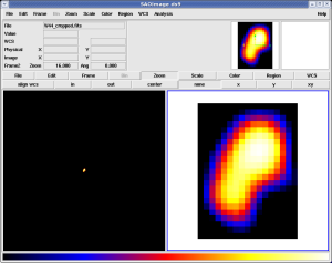
The FITS file on the left is 1000x1000 pixels most of which are zero. This is almost optimally bad. Except for events lying right on the source, the diffuse response integrals are almost all zero. The image on the right is the same data, but cropped to the 17x23 pixel region that actually contains relevant data. Performing an unbinned likelihood fit using this smaller map produces accurate results even in the presence of significant Galactic diffuse emission.
Analysis object creation using the hoops/ape interface
The UnbinnedAnalysis and BinnedAnalysis modules contain functions that use the hoops/pil/ape interface to take advantage of the gtlike.par file for specifying inputs. Usage of this interface may be more convenient than creating the UnbinnedObs, UnbinnedAnalysis, BinnedObs, and BinnedAnalysis objects directly. Here are some examples of their use:
- In this example, the call to the unbinnedAnalysis function is made without providing any arguments. The gtlike.par file is read from the user's PFILES path, and the various parameters are prompted for just as when running gtlike (except that the order is a bit different). If one is using the ipython interface with readline enabled, then tab-completion works as well.
>>> from UnbinnedAnalysis import *
>>> like = unbinnedAnalysis()
Response functions to use[P6_V1_DIFFUSE]
Spacecraft file[test_scData_0000.fits] test_scData_0000.fits
Event file[filtered.fits] filtered.fits
Unbinned exposure map[none]
Exposure hypercube file[expCube.fits]
Source model file[anticenter_model.xml]
Optimizer (DRMNFB|NEWMINUIT|MINUIT|DRMNGB|LBFGS) [MINUIT]
>>> like.model
Crab
   Spectrum: PowerLaw2
0       Integral:  1.540e+01  0.000e+00  1.000e-05  1.000e+03 ( 1.000e-06)
1          Index: -2.190e+00  0.000e+00 -5.000e+00  0.000e+00 ( 1.000e+00)
2     LowerLimit:  2.000e+01  0.000e+00  2.000e+01  3.000e+05 ( 1.000e+00) fixed
3     UpperLimit:  2.000e+05  0.000e+00  2.000e+01  3.000e+05 ( 1.000e+00) fixed

Geminga
   Spectrum: PowerLaw2
4       Integral:  1.020e+01  0.000e+00  1.000e-05  1.000e+03 ( 1.000e-06)
5          Index: -1.660e+00  0.000e+00 -5.000e+00  0.000e+00 ( 1.000e+00)
6     LowerLimit:  2.000e+01  0.000e+00  2.000e+01  3.000e+05 ( 1.000e+00) fixed
7     UpperLimit:  2.000e+05  0.000e+00  2.000e+01  3.000e+05 ( 1.000e+00) fixed

PKS 0528+134
   Spectrum: PowerLaw2
8       Integral:  9.802e+00  0.000e+00  1.000e-05  1.000e+03 ( 1.000e-06)
9          Index: -2.460e+00  0.000e+00 -5.000e+00  0.000e+00 ( 1.000e+00)
10    LowerLimit:  2.000e+01  0.000e+00  2.000e+01  3.000e+05 ( 1.000e+00) fixed
11    UpperLimit:  2.000e+05  0.000e+00  2.000e+01  3.000e+05 ( 1.000e+00) fixed
- Alternatively, one can give all of the parameters explicitly. This is useful for running in scripts.
>>> like2 = unbinnedAnalysis(evfile='filtered.fits', scfile='test_scData_0000.fits', irfs='P6_V1_DIFFUSE', expcube='expCube.fits', srcmdl='anticenter_model.xml', optimizer='minuit', expmap='none')
- The mode='h' option is available as well. In this case, one can set a specific parameter, leaving the remaining ones to be read silently from the gtlike.par file.
>>> like3 = unbinnedAnalysis(evfile='filtered.fits', mode='h')
- A BinnedAnalysis object may be created in a similar fashion using the binnedAnalysis function:
>>> from BinnedAnalysis import *
>>> like = binnedAnalysis()
Response functions to use[P6_V1_DIFFUSE::FRONT]
Counts map file[smaps_0_20_inc_front.fits]
Binned exposure map[binned_expmap_0_20_inc_front.fits]
Exposure hypercube file[expCube_0_20_inc.fits]
Source model file[Vela_model_0_20_inc_front.xml]
Optimizer (DRMNFB|NEWMINUIT|MINUIT|DRMNGB|LBFGS) [MINUIT]
Photon and Energy Flux Calculations
With Likelihood v13r18 and pyLikelihood v1r6 (ST v9r8), a facility has been added for calculating photon (ph/cm^2/s) and energy (MeV/cm^2/s) fluxes over a selectable energy range. The errors on these quantities are computed using the procedure described in this presentation made at the September 2008 Collaboration meeting. Here are some usage examples:
>>> like.model
Extragalactic Diffuse
   Spectrum: PowerLaw
0      Prefactor:  7.527e-02  7.807e-01  1.000e-05  1.000e+02 ( 1.000e-07)
1          Index: -2.421e+00  1.968e+00 -3.500e+00 -1.000e+00 ( 1.000e+00)
2          Scale:  1.000e+02  0.000e+00  5.000e+01  2.000e+02 ( 1.000e+00) fixed

GalProp Diffuse
   Spectrum: ConstantValue
3          Value:  1.186e+00  5.273e-02  0.000e+00  1.000e+01 ( 1.000e+00)

Vela
   Spectrum: BrokenPowerLaw2
4       Integral:  9.176e-02  3.730e-03  1.000e-03  1.000e+03 ( 1.000e-04)
5         Index1: -1.683e+00  5.131e-02 -5.000e+00 -1.000e+00 ( 1.000e+00)
6         Index2: -3.077e+00  2.266e-01 -5.000e+00 -1.000e+00 ( 1.000e+00)
7     BreakValue:  1.716e+03  2.250e+02  3.000e+01  1.000e+04 ( 1.000e+00)
8     LowerLimit:  1.000e+02  0.000e+00  2.000e+01  2.000e+05 ( 1.000e+00) fixed
9     UpperLimit:  3.000e+05  0.000e+00  2.000e+01  5.000e+05 ( 1.000e+00) fixed

>>> like.flux('Vela', emin=100, emax=3e5)
9.2005203669330761e-06

>>> like.flux('Vela')
9.2005203669330761e-06

>>> like.fluxError('Vela')
3.73060211564e-07

>>> like.energyFlux('Vela')
0.0047870395747710718

>>> like.energyFluxError('Vela')
0.000260743911378
The default energy range for the flux and energy flux calculations is (emin, emax) = (100, 3e5) MeV. Either or both of these may be set as keyword arguments to the function call. The errors are available as separate function calls and require that the covariance matrix has been computed using "covar=True" keyword option to the fit function:
>>> like.fit(covar=True)