Energy Dispersion Approximations
- Current (ST-09-25-02 and earlier) latResponse::Edisp2 does not interpolate the energy dispersion parameters from the IRF tables. This is because the parameters do not vary smoothly from bin to bin in log10(E)-cos(theta) space.
- It does apply a scale factor to the fractional energy difference, (Emeas - E)/E, that is a continuous function of log10(E) and cos(theta):
scaleFactor = p0*log10(E)**2 + p1*cos(theta)**2 + p2*log10(E) + p3*cos(theta) + p4*log10(E)*cos(theta) + p5
The p[0-5] are determined empirically (and hardcoded since P6 at least!) to make the 68% containment "radius" in energy space be approximately 1, independent of energy. - In order to have a properly normalized energy dispersion function, application of this scale factor forces the standard implementation to renormalize the Edisp2 function for every function call that requests a log10(E)-cos(theta) pair that differs from the previous function call. This is computationally costly, but it did not matter much for just making performance plots (presumably, this would impact running gtrspgen.)
- The calls to Edisp2 are contained within the DRM generation, and that step can take a substantial amount of time. In order to speed that up, the scaleFactor(log10(E), cos(theta)) function is only evaluated at the grid points, the normalization parameters in the Edisp tables are adjusted, and when function calls to Edisp2 are made, the nearest log10(E)-cos(theta) grid points are used, just as for the Edisp parameters themselves.
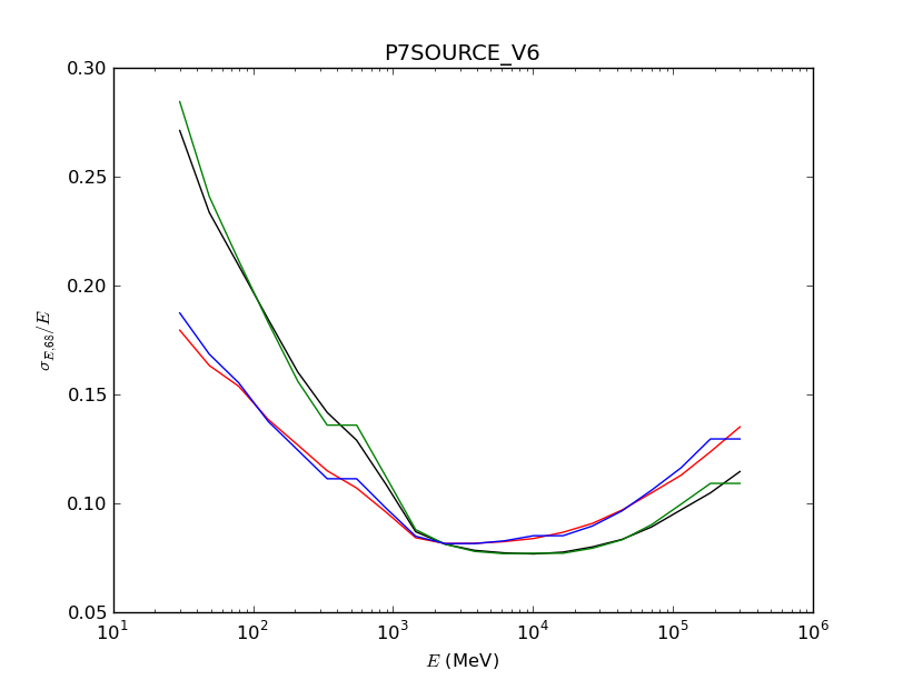
- Here is the impact on one of the standard performance plots:

black=Front, red=Back, both with scaleFactor as a continuous function of log10(E), cos(theta); green=Front, red=Back, both with scaleFactor evaluated at the nearest log10(E)-cos(theta) grid point.
Detector Response Matrix (DRM) Implementation
The DRM is the linear matrix that transforms a binned counts spectrum from true energies to measured energies:
\begin
n_
= \sum_k D_
n_k
\end
where
$n_
$
are the counts in measured energy bin
$k^\prime$
and
$n^k$
are the counts in true energy bin
$k$
.
\begin
D_
= \frac{\int_{\Delta E_{k^\prime}} dE^\prime \int d\theta d\phi D(E^\prime; E_k, \theta, \phi) A(E_k, \theta, \phi) lt(\theta, \phi)}
\end
Here
$D(E^\prime; E, \theta, \phi$)
is the energy dispersion function,
$A(E, \theta, \phi)$
is the effective area, and
$lt(\theta, \phi)$
is the integrated livetime as a function of detector coordinates associated with the specified sky position. The integral over measured energy is taken over the width of the
$k^\prime$
bin. This follows the DRM calcuation in gtrspgen![]() .
.
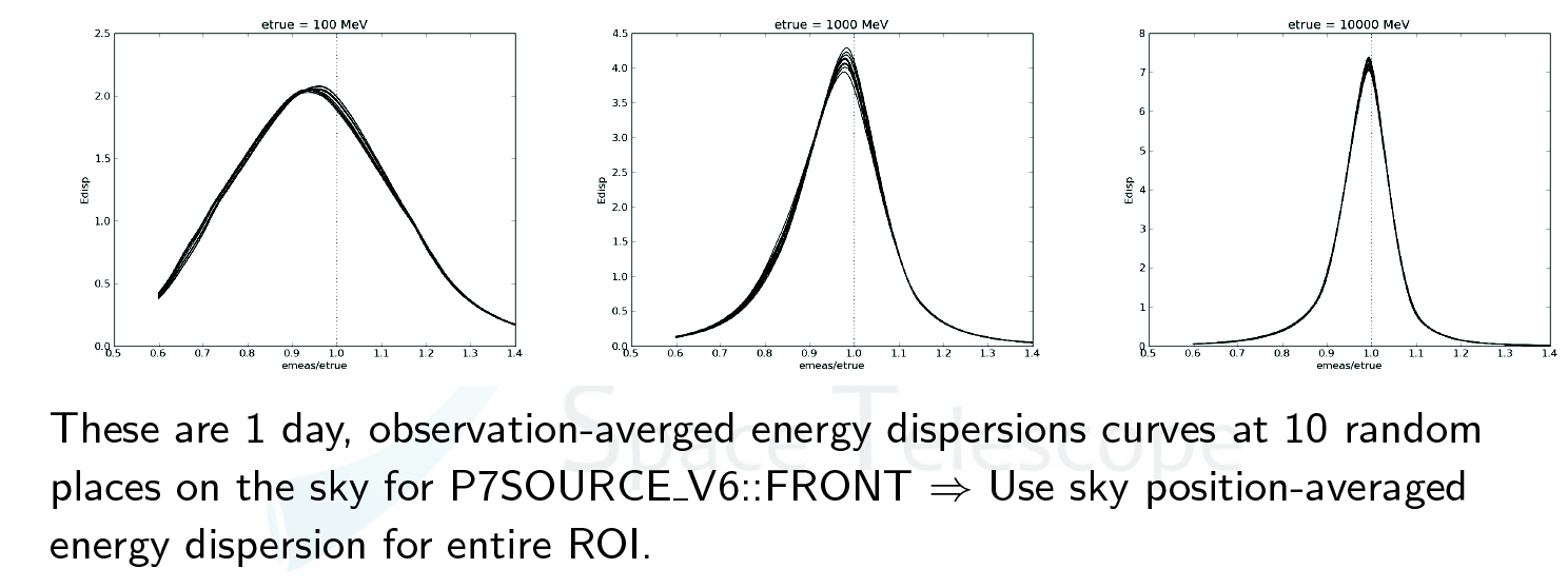
In princple, the DRM should be evaluated at each sky pixel position in the binned counts map, but we make the approximation that the DRM does not change much over the counts map region and just evaluate it at the map center and assume it applies everywhere on the map. This is supported by these plots of the energy dispersion evaluated at various points on the sky for a one-day survey mode integration: