Page under construction.

This page summarize the main points of the analysis I did on HESS J1857+026 using 2 sample of data.

The first analysis used 31 months of data collected from August 4, 2008, until March 2011. Only gamma-rays in the Diffuse class events were selected and we excluded those coming from a zenith angle larger than 100°.We have used the P6_V11_Diffuse instrument response functions (IRFs). We included in the model all the sources of the 18 month catalog and assiociated diffuse files.

The second analysis used the same amount of data. Only gamma-rays in the source class events were selected and we excluded those coming from a zenith angle larger than 100°. We have used the P7_V6_SOURCE IRFs. We included in the model all the sources of the 2FGL catalog and assiociated diffuse files.

The Region of Interest.

HESS J1857+026 is in the same region than the SNR W44 which is the brightest source of the region.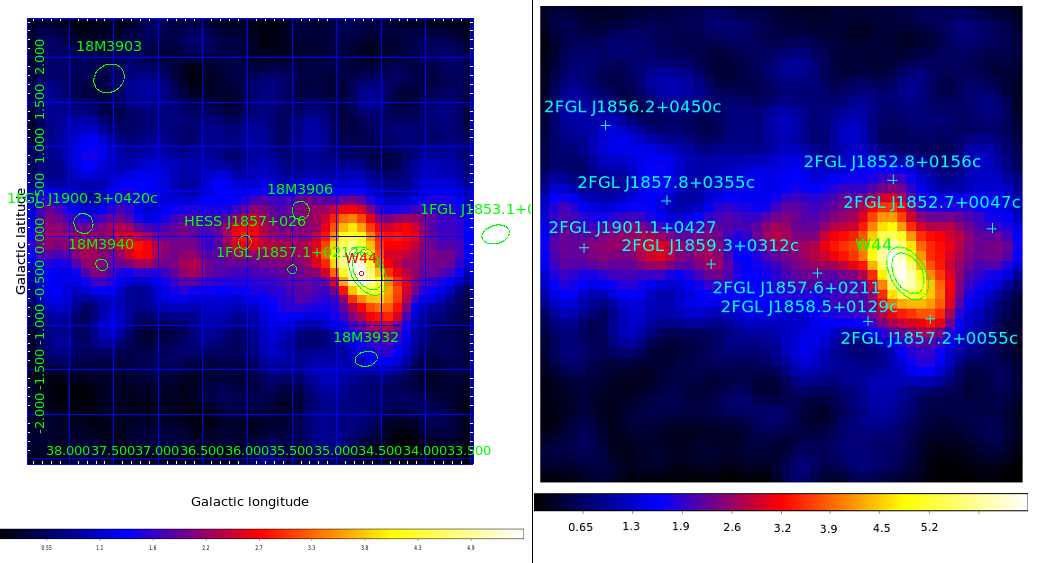

Fig 1. Counts map of the region above 6 GeV. Left Pass 6 analysis with 18 months catalog sources in green. Right : Same picture corresponding to the Pass 7 analysis with 2FGL sources represented in blue.

W44

The shape of W44 was fitted by an Elliptical Ring (ref. 1) and it spectra by a broken power law.

We saw an excess close to W44 and tried to refit the source to take into account this excess.

We refitted again the spectra of W44 by a Log-Parabola and studied the shape of W44.

The main point is that the results are consistent with previous work and with 2FGL cat.

 
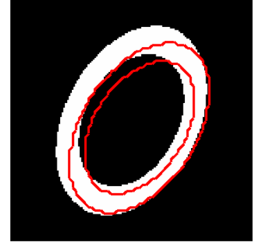
Fig. 2. Comparison between the result of ref. 1 (red contours) and our results using pass 6 (white ring) . There is no error taken into account in this templates. Figure to be updated with Pass 7

Table 1.  Parameters obtained by fiting the shape of W44. The main point is that all of these values are consistent with the work of Tanaka et al. 2010.

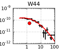
Fig. 3 SED of W44 given by pointlike.

Adding a new source to Pass 7 Analysis

section under construction

Using 2FGL sources, Pass 7 IRFS and associated diffuses, we found a low energy excess quickly decreasing with energy.

To prevent contamination from this source on HESS J1857 we analysed it. The best fit we obtained is a point source located at 

RA=283.58 DEC=2.98

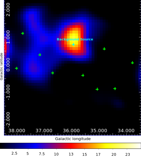
Fig. 4. Residual TS map between 100MeV and 1.3GeV using pointlike. Green crosses represents 2FGL sources

 
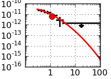
Fig. 5. SED of the source using pointlike.

The best fit using gtlike provided the following parameters and statistical errors alpha = 3.5 +/- 0.2, beta = 0.6 +/- 0.1, Eb ? 1.2 GeV, and N_0 = (3.1 +/- 0.5) X 10^{-12} photons/MeV/cm^2/s.

Search for pulsed emission

A.LYNE, B. STAPPERS and C.ESPINOZA kindly provided us timing solution of PSR J1856+0245 which powers HESS J1857+026.

Marie-Helene searched for pulsation concidering 43 pulsars in 3° around the HESS position but found no pulsed emission from PSR J1856+0245. H-Test <<2.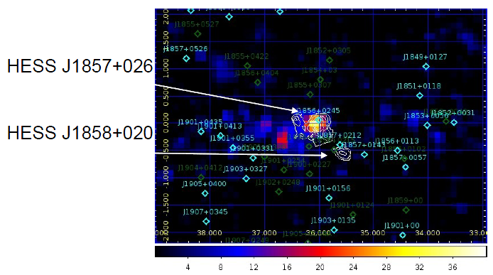
Fig.6 TS map above 10GeV using Pass6_V11. HESS J1857 is not included in the model. white contours are those obtained using HESS data. Cyan : Pulsars monitored by radio-telescopes. Green : Other pulsars (from the ATNF database)

Only one good candidate was found :  PSR J1856+0113 located in W44 :

 
Fig. 7. Light curves and H-Test obtained looking at PSR J1856+0113  above 50 MeV and 300MeV.

HESS 1857+026 Morphology above 10GeV

To avoid any contamination from other sources or diffuse emission from the Galactic plane we tested for extension above 10 GeV. All the sources previously announced were taken into account (18 months -> Pass 6, 2FGL +1 ->Pass 7).

Table 2. TS and Loglike found above 10GeV for a point source, a gaussian and a Disk. Pass 6 analysis.

Table 3. TS and Loglike found above 10GeV for a point source, a gaussian and a Disk. Pass 7 analysis.

Table 4. Fited positions.

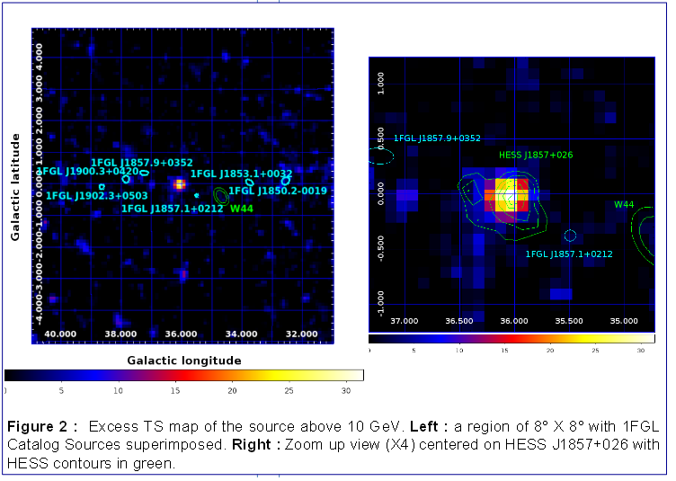
Fig. 8. Residual TSMap in which HESS J1857 is not fitted. Pass 6 analysis. + HESS contours

Fig 9. Residual TSMap in which HESS J1857 is not fitted. Pass 6 analysis. + HESS contours. Green crosses represents 2FGL sources.

Spectral analysis

We fitted the source using pointlike above 300GeV to prevent contamination at low energy.

Here are the summary of the Pass 6 analysis :

The best fit obtained using pointlike gave the following parameters :

Table. 5. Parameters of the best fit obtained using pointlike on Pass6.

Those gave the following SED :

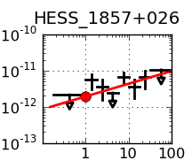
Fig. 10 SED obtained with pointlike using Pass 

The following SED and best fit are those obtained using Pass 7 :

 
Fig. 11 : SED obtained using gtlike above 300 MeV. The best fit is shown in yellow.

The source is fitted by a hard power law. The parameters of the best fit are those of the next table :

Table. 6. Parameters of the best fit obtained using gtlike.

SED modeling

Section under construction

Adam constructed a time-dependent one-zone SED model with constant expansion velocity, and assuming a distance of 9 kpc. The modeling only need an IC component.

Fig. 12 show the SED modeling constructed by Adam. Blue point are those obtained with HESS data and the green one using ASCA observation. IC components : stellar (dot), IR (medium-dashed) and scattering on
CMB (long-dashed)
Preliminary fit:

Final B = 1.5 ± 1.0 ?G
Electron slope = 2.2 ± 0.1
Electron cutoff = 120 ± 40 TeV
Initial spin period = 13 ± 8 ms
Braking index = 2.5 ± 0.4

Theses parameters predict an age of 25 kyrs (21 kyrs predicted in Hessels et al. 2008 for the pulsar).

Discussion

Assuming a distance of 9kpc we derived the luminosity of the PWN to compute its gamma efficiency. We obtained :

L? (PWN) = 1.69 X 10^35 ergs/s.

Using the pulsar Edot =4.6 X 10^36 we computed an efficiency of 3.7%. To compare to the 3.1% obtained using HESS data.

This efficiency is consistent with what is expected from Ackerman et al. 2011 (the order of magnitude of the percent) as is shown in the following picture :

Fig. 13 ?-ray Luminosity of the Pulsar Wind Nebulae as a function of the spin-down
luminosity of the associated pulsar. All the pulsar wind nebulae detected by Fermi are
associated with young and energetic pulsars. Pulsar wind nebulae detected by Fermi are
marked with red stars. Blue squares represent pulsars for which GeV ?-ray emission
seems to come from the neutron star magnetosphere, and not from the nebula.

With more data

To compare our spectral points to those obtained with MAGIC (talk at the ICRC Klepser et al., Mapping the extended TeV source HESS J1857+026 down to
Fermi-LAT energies with the MAGIC telescopes) we reanalyzed the source to 300 MeV using more data (36 months instead of 31). Here are the results obtained :
Fig. 14 Residual TS map obtained between 10GeV and 300GeV. Here HESS J1857 is not included in the model. The green contours are those obtained using HESS data (Aharonian et al.,2008).

The position of the Fermi excess is consistent with those of HESS. The black circle represents the position of PSR J1856+0245.

Table 7: Best fit parameters for 36 month of data fitting between 300MeV and 300GeV.

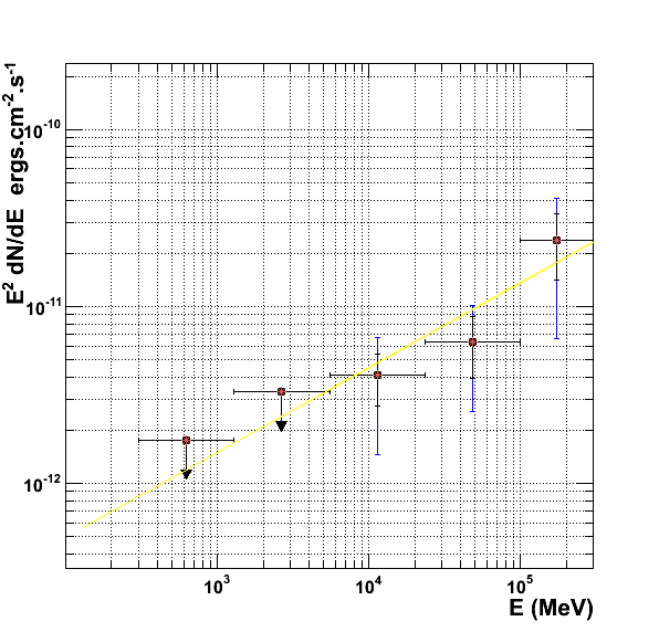
Fig. 15 : SED obtained using gtlike above 300 MeV. The best fit is show in yellow. Statistic and systematics error bars are respectively the black and blue lines.

We added one source of systematics using a template consistent with those of HESS data (Aharonian et al.,2008). The SED thus obtained is consistent with the one shown by Klepser et al. at the ICRC.

Using our model we derived and upper limit on the DC emission of the pulsar :

F(100MeV-100GeV)< 9.77×10?9 ph/cm2/s leading to a limit on the gamma-ray luminosity of 8.27 × 1035erg/s.

In the paper

I'm now writting the draft of an A&A letter with M.-H. Grondin, M. Lemoine-Goumard, A.Van Etten, B. Stappers, A. Lyne, C. Espinoza.

The first part is an introduction of the source.

The second part summarize the data I used.

The third part (Fermi data analysis) is divided in 2

1. Search for pulsation. -> No pulsed emission
2. Spatial and spectral analysis

• Spatial
• Spectral

The discussion begins with the SED modeling and present the gamma-ray luminosity and efficiency.

I would like to show 3 figures which are th Fig. 4, 14 and 16(comming soon).

The draft is coming soon.

Bibliography :

(1) Abdo et al., Science,327, 1103-1106, 2010

(2) Hessels et al., ApJ, 682, L41-L44, 2008
(3) Aharonian et al., A&A, 477, 353-363, 2008

(4) Cordes, J. M., & Lazio, T. J. W. 2002, preprint (astro-ph/0207156)
(5) Vincent, M., Thesis : “Nebuleuse de pulsars : sondage profond de la Galaxie au TeV et études multi-longueur d'onde”.

(6) Sugizaki et al., ApJ Supplement Series, 134, 77-102, 2001

(7) Ackermann et al., ApJ, 726, 35-102, 2011