This is an unmodified version of exercise 4 from the 2005 Cern School of Computing. With some cleanup it could be made into a introduction to SLIC/LCDD. The code for the exercise is attached.
Simulation, Visualization, and Analysis
Exercise 4 - GDML, Analysis & Visualization
Introduction
In this exercise we will demonstrate the use of an XML file to configure Geant4 geometry. As described in the lectures, we will use LCDD, an extension of the standard Geant4 GDML format to describe a complete detector setup, including sensitive detectors and readout. Since we are using XML to configure Geant4 there is no need to write any C++ code for this exercise, so we can use a version of Geant4 which has been pre-built with support for GDML included. This has been installed on all of the CSC workstations, and can be started simply by typing:
slic
at the command prompt. Issuing this command will cause a list of options to be displayed on the console. The following links give background information on the SLIC program, although this should not be needed for this exercise:
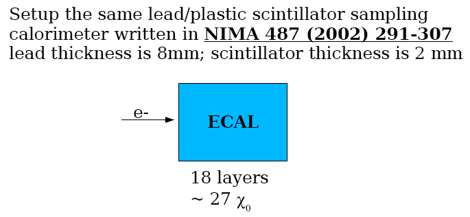
Although SLIC can be used to set up arbitrarily complex detector geometries this typically involves more work than we have time for in this exercise, so instead you will set up a simple test calorimeter, corresponding to that described in this NIMA 487 (2002) 291-307. The detector you will set up consists of 18 layers, each 1m square in the xy direction, with 8mm of lead followed by 2mm of plastic scintillator in the z direction. The scintillator is read out using photomultipliers, and thus represent the "sensitive" part of the calorimeter. We will simulate the effect of firing electrons at various energies into the front of the calorimeter. The goal of the exercise is to write out a file containing the simulated "hits" in the sensitive layers, and then to analyze this file to determine the energy resolution of the calorimeter for various electron energies.
Calorimeter Energy Resolution
Calorimeters of the type we are simulating here typically consist of a set of layers each consisting of a sandwich of an energy absorber made of a un-instrumented dense material (lead in this case), and a sensitive material (plastic scintillator) in which energy deposition is measured. The dense material causes incident particles to interact producing a shower of decay products. Ideally the entire energy of these decay products is deposited in the calorimeter, but only a small fraction of that energy is deposited in the sensitive material, and thus only a small proportion of the energy is measured. Since the showering process is random, for a given initial particle energy the proportion of the energy measured will vary randomly around some mean. The measured width of this random distribution is called the energy resolution, as is typically expressed in terms of ?E/E where ?E is the measured width of the distribution, and E is the mean energy deposited. ?E/E typically varies approximately linearly with ?E and so in this exercise we will make plots of ?E/E (in %) vs ?E to determine the energy resolution of our simulated calorimeter.
Setting up and Verifying the Geometry
Typing in the XML for this calorimeter from scratch still takes some time, so we have provided you with a starting point, which can be found in
~/simex/ex4/ecal.lcdd
This file has a deliberate mistake in it, so as part of the exercise you will use SLIC to simulate one event and view it with the WIRED4 event display. From the event display you should be able to figure out what the error is, and fix it.
To run slic to read the ecal.lcdd file and to generate a heprep file representing a single event use the following command:
cd ~/simex/ex4
slic -g ecal.lcdd -m vis1.mac
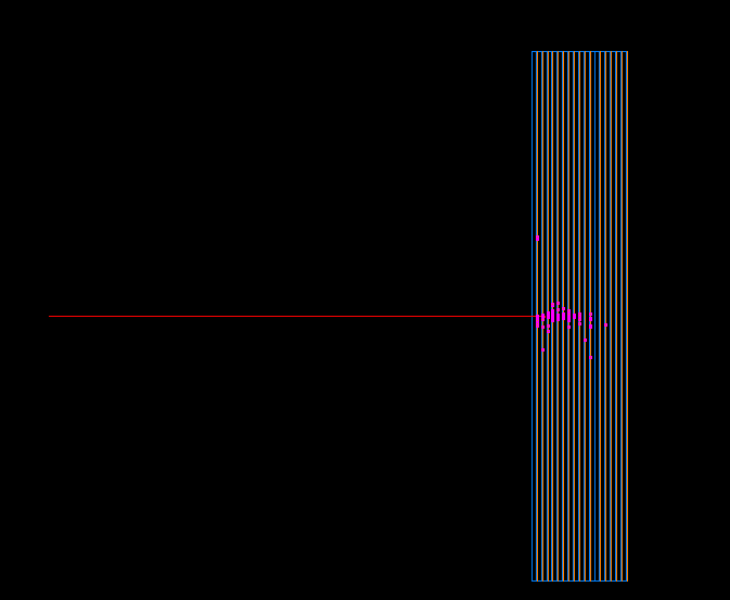
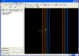
vis1.mac is a Geant4 macro which sets appropriate visualization options and sets up the standard geant4 "gps" particle gun to fire a single electron into your test calorimeter (however it may also have a deliberate mistake in it). Executing the above command causes a file scene-0.heprep.zip to be created. You can view this file by opening it using JAS3 and WIRED4 (see exercise 2 for instructions on opening heprep files with WIRED4) and after you find and fix the deliberate mistakes you should see something like this:
Editing XML files
XML files are plain ASCII file so they can be edited with any editor, however it is a good idea to use an editor which "understands" XML. There are many such editors available, we have pre-installed one open-source editor called "jedit" on the CSC computers. If you want to try this editor just use the command:
jedit ecal.lcdd
jedit provides many plugins, and we have preinstalled the XML plugins, which automatically read the XML schema for a particular XML file, and will highlight any illegal syntax in your XML file. This enables you to catch XML errors as soon as you save the file, which is much quicker than waiting until Geant4 discovers the errors. (Note the first time you open an XML file with jEdit it will ask if you want to download the schema, to which you should reply yes – unfortunately the LCDD schema consists of about 10 nested files, so you will have to answer yes about 10 times!)
Particle trajectories in Geant4
In the event display above you will only see the trajectory of the initial particle fired by the GPS gun into the calorimeter. It will stop somewhere near the entrance to the calorimeter, as it interacts and forms secondary particles. Since a shower consists of many secondary particles we do not normally keep the trajectories of all these particles, as they increase the size of the output file, and slow down Geant4. You can change this behaviour by setting store_secondaries=true in the DetectorRegion in your ecal.lcdd file, in which case you would see something like this:
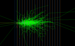
Make sure to set store_secondaries=false when generating the data files below.
Generating Data Files
Once you have found and corrected the errors in the LCDD file you can proceed to generate some simulated test beam data. We want to generate 500 events at each of a 1, 2, 4, 8, 16 GeV. (Ideally we would use more events and go to higher energies, but the simulation takes exponentially more time the higher the electron energy is, so to keep things simple we will only use these relatively low energies.)
We have provided a macro file which will run a two energies, ecal.mac. It should be obvious how to modify this macro to create electrons at each of the energies required. As before you can run slic with this macro by issuing the command:
slic -g ecal.lcdd -m ecal.mac
If things go correctly this should create a data file called ecal_e-.slcio containing all of the hits in the sensitive detectors for each event. If you used the recommend number of events and event energies the size of the created file should be about 9Mbyes and should take Geant4 about 10 minutes to create.
Viewing the Data Files in JAS3/WIRED4
In the next part of the exercise we will verify that we can read the data files using JAS3 and WIRED4.
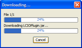
As mentioned in the lectures JAS3 is a modular analysis framework which can be extended in various ways by adding additional plugins. Before we will be able to open the LCIO file produced by Geant4, we must install the LCIO plugin for JAS3. To do this start JAS3, select "View", "Plugin Manager" from the menu bar. Now in the Plugin manager click on the "Available" tab, and select hep->linearcollider->lcio->LCIO (LCIO plugin for JAS3) from the available plugin tree, and then click on "Install selected plugins".
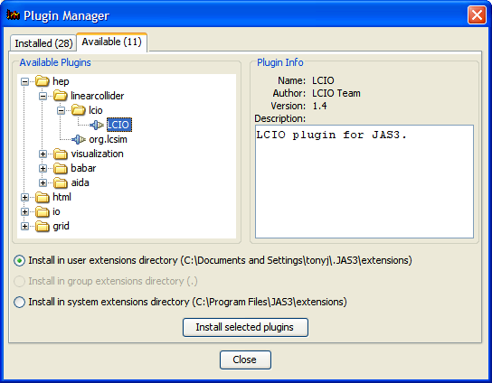
The LCIO plugin should be automatically downloaded from the web and installed.
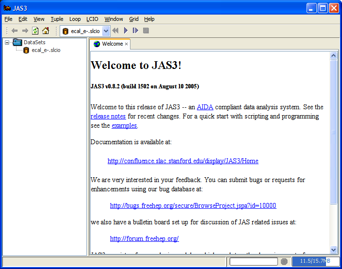
You can now close the plugin manager and open the data file (which should be called ecal-e-.slcio) using the "File", "Open File" menu item in the JAS3 menu bar. Once you open the file it should appear in the JAS3 tree, and a new item should appear in the JAS3 toolbar, allowing you to step through events. You can check that the file contents looks reasonable using two tools, the LCIO Event Browser, and the WIRED4 event display.
To use the Event Browser step to the first event (using the  button in the tool bar) and then from the LCIO menu select "Event Browser".
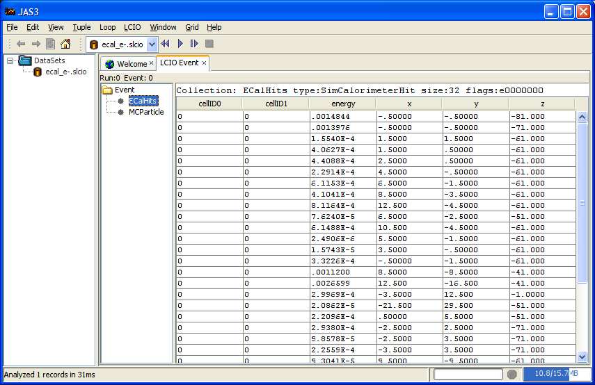
You should be able to verify that for each event the LCIO file contains an event header, the trajectory of the incoming electron, and the list of hits in the calorimeter.
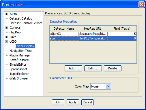
You can also use the WIRED event display to view the events. Since the events only contain the hits and particle trajectories but no detector geometry information you will first have to tell Wired where the heprep file corresponding to the detector is located. To do this select View, Preferences then in the preferences dialog tree select LCIO->Event Display. Now click Add, and enter the following information:
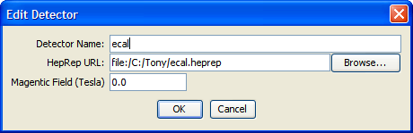
The detector name should be set to ECAL (the name given to the detector in the LCDD file, and stored in the event header of the LCIO file), the HepRep URL should be the path to the ecal.heprep file in your ~/simex/ex4 directory (use the Browse... button to locate this file) and the Magnetic Field should be set to 0 (since there is no magnetic field for this test detector).
After you click OK the settings should be added to the list of known detectors in the preferences dialog:
Now you should be able to select "File", "New", "WIRED4 View" in JAS3 and view the event. You should be able to step through different events to see how they look.
Analyzing the Data Files using JAS3
We have provided a simple analysis routine written in Java which can be used to analyze the LCIO file created in the previous section. The file will be in your ~/simex/ex4 directory:
~/simex/ex4/ECalAnalysis.java
The file is mostly complete, but one section, marked *** has been left for you to complete. The comments in the file give suggestions on how to do this. To run this file using JAS3 you need to do the following:
- Open the file using the "File", "Open File" menu item. The file will open in the JAS built-in editor (but you can use a different editor if you like to edit the file).
- Compile the file using the JAS compiler. The easiest way is to right-click on the JAS built-in editor and choose "Compile" from the popup menu.
- Load the program into memory using the "Load" item on the JAS popup menu.
- If you have not already done so, open the ecal_e-.slcio file using the "File", "Open File" menu item. If you have already opened the file make sure you are at the beginning of the file by choosing the "Rewind" item from the "Loop" menu.
- Now analyze the data by choosing "Go" from the "Loop" menu. The data will be read, and each event in turn will be passed to the recordSupplied() method of your analysis code. As histograms are created and filled they will appear in the JAS3 tree. You can double-click on the icons corresponding to histograms in the tree to view them, or use the popup-menu on the JAS3 tree to arrange multiple plots on the page.
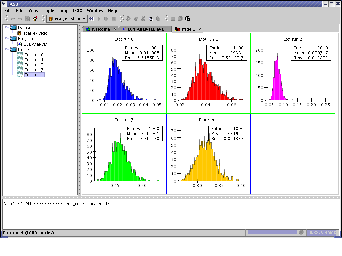
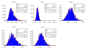
After you have analyzed all of the events you should have one histogram of total energy deposited in the calorimeter for each electron energy you generated with Geant4. Your plots should look something like this:
Producing a Plot of the Energy Resolution vs. Energy
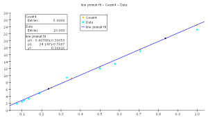
The final step in the analysis is to perform a fit to each energy distribution, to compute the measured energy resolution at each incident electron energy. We will fit a Gaussian function to each of the histograms we produced to compute the mean and sigma of the distribution, and we can then compute the energy resolution as sigma/mean. To compare to the published data we can then produce a plot of energy resolution (in percent) vs sqrt(electron energy), and compare to the published data tabulated below.
You have the choice of performing this part of the analysis using either Java, Python or Pnuts (a simple to learn Java-like scripting language). We have provided templates for the solution in each language in the ~//ex4 directory:
- Fit.java (Java). To use this file open the file in JAS, compile and load as before, then choose "Run" from the editor popup menu to run it.
- fit.py (Python). To use this file open the file in JAS, and choose Run from the editor popup menu (no need to compile or load)
- fit.pnut (Pnuts). To use this file open the file in JAS, and choose Run from the editor popup menu (no need to compile or load)
Once again one part of the file, marked *** has been left for you to fill in. Comments in the file give hints on how to do this.
You should produce plots which look something like the following plots:
Additional Exercises
In the unlikely event that you got this far, still have time left, and for some reason don't feel like going to the beach, here are a few more ideas to experiment with:
- Try changing the material in the calorimeter (say from lead to tungsten) or changing the relative widths of the sensitive/insensitive layers to see what effect this has on the resolution.
- Try firing pi- instead of e- into the calorimeter. In this case you will need many more layers in the calorimeter. Try hcal.lcdd instead of ecal.lcdd as the detector definition.