Background
Josh Lande recently ran some consistency tests comparing the Monte Carlo point source parameters to the values fit by binned likelihood for point sources. For the spacecraft data, he used a one-day interval of the idealized +/-50 deg rocking provided by gtobssim. For one location on the sky, location 0: (RA, Dec) = (176.31, 44.28), the fitted flux in the 0.1-100 GeV band was too high relative to the MC value by ~8%, whereas at location 1: (RA, Dec) = (-176.31, -44.28), the disparity appeared negligible.
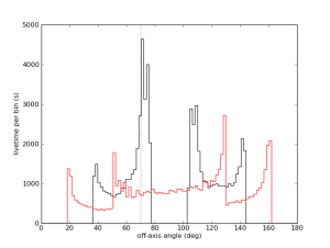
For such a short time scale (1 day), these two sky locations have very different off-axis profiles. Here are histograms of the livetime as a function of off-axis angle for the two locations. The black histogram corresponds to location 0, and the red corresponds to location 1.
Diagnosis
The bug lay in the code that computes the exposure averaged PSF. This is given by

Here  and
and  are the PSF and effective area, respectively, and
  is the angle of the source relative to the instrument z-axis. The phi-dependence of
  and
and  is suppressed for clarity.
  is the angle between true and measured photon direction, and
  is the photon energy. In the second line of the above equation, the integrals have been recast as integrations over theta. These integrations are performed using the livetime cubes computed with gtltcube.
In ST-09-27-01 and earlier, there is a cutoff at theta=70 deg for the mean PSF calculation. The original reason for this cutoff is unclear, but it was probably motivated by some poor behavior of the PSF at large theta angles for an early version of the IRFs. As far as the shape of the PSF is concerned, this truncation does not have a significant effect. As part of some recent refactoring, this truncation was removed in Likelihood-17-22-04 (22 Feb 2012).
Unfortunately, I had thought that the truncation only affected the PSF shape calculation. In fact, for point sources, the binned analysis code has been using the exposure calculation in the denominator of the mean PSF expression for computing the model counts rather than using the exposure from the binned exposure map. Hence, all point source fits will be affected by this truncation. For location 0 (black histogram in above figure), a significant fraction of its time is spent just beyond the theta=70 deg cutoff. This is the cause of the 8% disparity that Josh found in his tests.
Effects
One can estimate the impact of the theta=70 deg cutoff by running gtexpcube2 with the option thmax=180 in the nominal case (this is the default) and thmax=70 in the truncation case. Assuming a photon index of -2, which Josh used in his gtobssim runs, one can estimate the expected fractional offset in measured flux (Fmeas) relative to the MC value (Fmc), (Fmeas - Fmc)/Fmc, using the spectrally weighted exposures, exposure , and computing (exposure180 - exposure70)/exposure70.
For the one-day simulation, here is a map of the estimated fractional offset in Galactic coordinates:
- One day
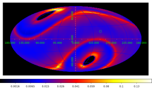
The green point near the Northern Galactic pole is location 0 and has a fractional flux offset of 8%, and the green point nearer the Galactic plane has flux offset of 1.5%. The peak offsets can be has high as 16.3%.
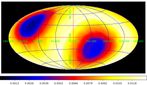
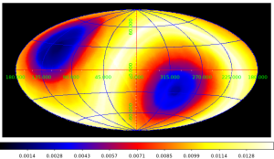
On longer time scales, these offsets are considerably smaller. Here are maps for the 18 month and 2 year livetime cubes used by the catalog group for 2FGL:
- 18 months (/afs/slac/g/glast/groups/catalog/P6_V8_DIFFUSE/ltcube_18months_rock52.fits)
- 2 years (/afs/slac/g/glast/groups/catalog/P6_V8_DIFFUSE/ltcube_2years_rock52.fits)
I've computed livetime cubes for 30 day intervals and have estimated the fractional offset as a function of time for the Vela, Crab, and Geminga pulsars.
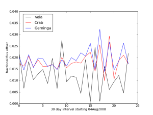
There is a DC offset of about 1.5% and an additional dispersion of about the same size. NB: These estimates assume a power-law spectrum with photon index -2 over the entire integration range 0.1-100 GeV.