Content
Psocake Layout
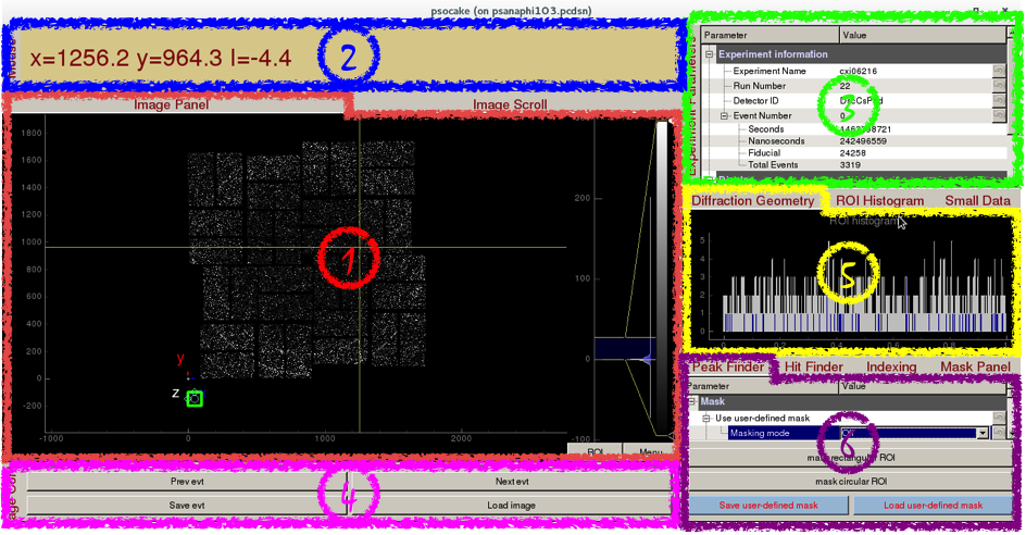
- Image Panel / Image Scroll
- Mouse Panel
- Experiment Parameters
- Image Control
- Diffraction Geometry / ROI Histogram / Small Data
- Peak Finder / Hit Finder / Indexing / Mask Panel
Experiment Parameters
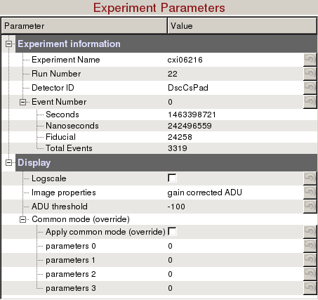
Experiment information requires 4 fields to uniquely identify a detector image:
- Experiment Name: Experiment name, (e.g. cxi06216)
- Run Number: Run number, (e.g. 22)
- Detector ID: The full name (e.g. CxiDs1.0:Cspad.0) or DAQ alias (e.g. DscCsPad) for the detector. Available area detector names are printed to Terminal when Experiment Name and Run Number are entered.
- Event Number: Event number starting from 0. Seconds, nanoseconds, fiducials and total number of events are read-only.
Display
- Logscale: Display detector image in logn scale.
- Image Properties: There are many image properties besides pixel readout values that can be displayed.
- Pixel readout
- gain corrected ADU: Pixel values after pedestal, common mode, and gain correction. Hybrid gain at CXI is also corrected. (Default display)
- common mode corrected ADU: Pixel values after pedestal and common mode correction.
- pedestal corrected ADU: Pixel values after pedestal correction.
- raw ADU: Pixel values without any correction.
- photon counts: This feature isn't implemented yet.
- Pixel correction
- gain: Gain correction values. Pixel values are calibrated by multiplying by the gain.
- common mode: Common mode correction values. Pixel values are calibrated by subtracting the common mode.
- pedestal: Pedestal correction values. Pixel values are calibrated by subtracting the pedestal.
- pixel_status: Status of each pixel determined from a dark run. Good pixel status is zero. Calibrated pixels that have bad pixel status are set to zero.
- pixel_rms: Root mean square of pixel values from a dark run.
- Pixel position
- quad number: Corresponding detector quadrant of the pixel (Quad,Seg,Row,Col)
- seg number: Corresponding detector segment of the pixel (Quad,Seg,Row,Col)
- row number: Corresponding detector row of the pixel (Quad,Seg,Row,Col)
- col number: Corresponding detector column of the pixel (Quad,Seg,Row,Col)
- coord_x: Pixel x-coordinates
- coord_y: Pixel y-coordinates
- Pixel readout
- ADU threshold: Threshold used for display purposes only (Default: -100 ADUs)
- Common mode (override):
- Apply common mode (override): Turn on/off common mode ignoring the values deployed in /reg/d/psdm/<instrument>/<experiment>/calib directory.
- parameter 0, 1, 2, 3: Parameters are described here --> Common mode correction algorithms. Once the common mode parameters have been optimized using psocake, you should deploy these parameters using Calibman, e.g. For a median algorithm with correction limits at 1000 ADUs (3, 1000, 1000, 128) or for an unbonded pixel algorithm #5 with correction limits at 50 ADUs (5, 50, 0, 0).
Image Panel / Image Scroll
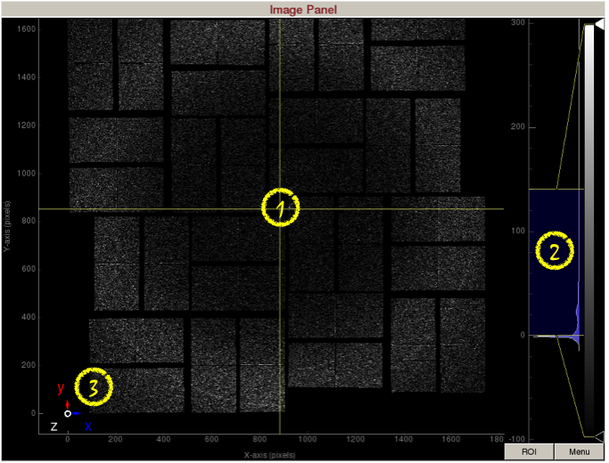 Image panel displays the detector image.
1) Display area shows the assembled detector image. This area can be panned by dragging with the mouse, and zoomed in/out using the middle mouse wheel.
2) Intensity histogram can be used to adjust image contrast. The intensity histogram can be zoomed in/out using the middle mouse wheel. The blue shaded area selects the region of the intensity histogram to display on screen. You can drag the blue shaded area up/down to change the maximum/minimum display values. You can also drag the two yellow horizontal bars up/down to change the maximum/minimum display values. The white and black triangles can be dragged up/down to change the mapping between pixel value and display color.
3) Coordinate marker shows the lab coordinates of the detector. Z-axis is coming out of the screen.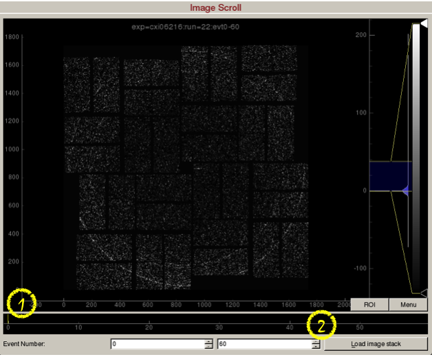
Image scroll is used for viewing a stack of images.
1) Scroll bar to set the event on display. Alternatively, press the spacebar to play/stop the movie.
2) "Load image stack" button will load 60 frames starting from event number 0. These values are adjustable.Mouse Panel

Mouse panel displays the pixel x-coordinates, y-coordinates, and intensity.
It will also display "Masking Mode", if masking mode is turned on.Image Control

Image control has 4 buttons.
Prev/Next evt: Click to goto previous/next event.
Save evt/Load image: Click to save/load a Numpy image of the detector.Diffraction Geometry
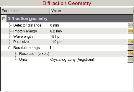
Diffraction Geometry can be used to optimize the detector distance and draw resolution rings:
- Detector distance: Sample to detector distance.
- Photon energy: Photon energy is automatically updated each event. It can be manually overridden.
- Wavelength: Wavelength is automatically updated when the photon energy is updated. (Read-only)
- Pixel size: Pixel size is automatically updated for some of the detectors. It can be manually overridden.
- Resolution rings: Check to display resolution rings on the image panel.
- Resolution (pixels): Enter radius in pixels, comma-separated for multiple rings.
- Units: Select the desired units of the resolution.
- Crystallography (Å/Nanometre/q)
- Physics (Å/Nanometre/q)
- Scattering Vector (2θ)
ROI Histogram
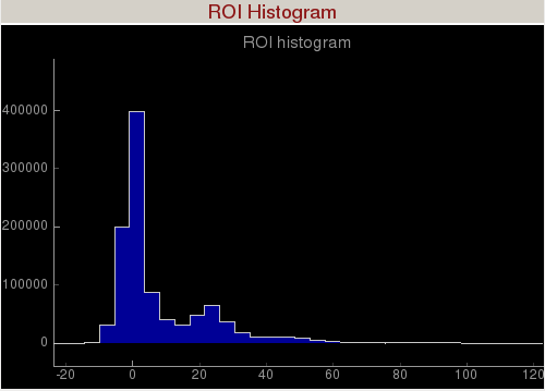
Region of Interest (ROI) Histogram panel histograms the pixel intensities inside the green square (shown in the figure below), green polygon, and green circle. The green ROI can be moved around (by clicking inside the ROI and dragging) to study the intensity distribution of a region of interest. You can zoom in/out of the plot using the mouse scroll or a two-finger slide up/down on a Mac track pad. You can reset the plot by clicking on "A" at the lower left corner of the plot. The diamond handles on the green ROI can be dragged to resize the ROI. The green square will display the ROI in assembled and unassembled shapes in your terminal. The green circle will display the centre position of the ROI in your terminal. You can add extra vertices in the green polygon by right clicking on an edge. (Left click on a vertex to remove it.)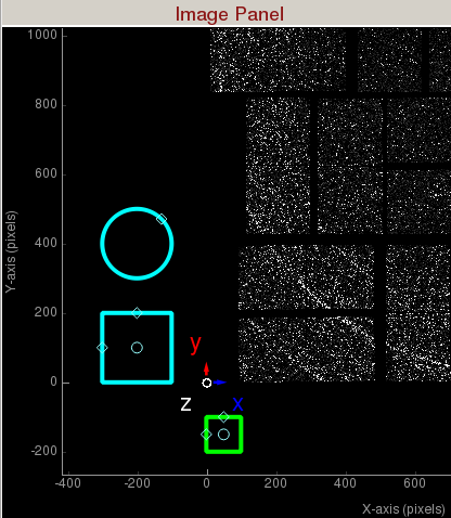
The green square is the region of interest for intensity histogramming. Note the cyan circle , cyan polygon, and cyan square are for mask generation.Small Data
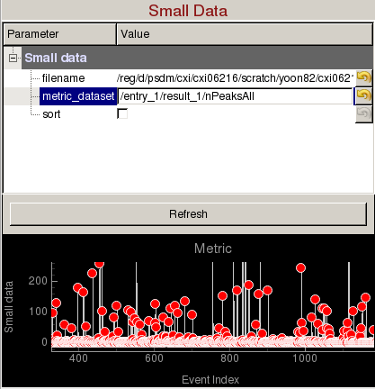
Small Data panel can be used to plot a metric vs event number and display images from specific events of interest:
- filename: Name of an hdf5 file (cxidb or NeXus files are OK).
- metric_dataset: Dataset inside the hdf5 file containing the small data. It is recommended that the small data is recorded for all events in the run. If not, then the hdf5 file needs to contain /event dataset to identify which events were recorded (e.g. If /entry_1/results_1/smallData is the dataset containing /entry_1/results_1/event is an array of event numbers with the same length).
- sort: Ascending sort of the small data. You can still click on the red markers to display the corresponding image.
Peak Finder
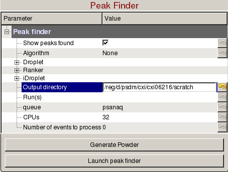
Peak Finder panel is used to tune peak finding parameters for detector images with peaks, generate powder patterns, and launch peak finding jobs on the computing cluster:
- Show peaks found: Check to display the peaks found.
- Algorithm: Select the peak finding algorithm. Documentation can be found here: Peak Finder Algorithms
- Droplet: peak_finder_v1
- Ranker: peak_finder_v3
- iDroplet: peak_finder_v4
- Droplet/Ranker/iDroplet: Click on the corresponding algorithm and adjust parameters. The peaks found on the detector will get updated.
- Output directory: Directory where the output hdf5 will be saved.
- Run(s): Comma separated list of run numbers to submit to the cluster, or colon for a range of runs, (e.g. 1,4:6,9 --> runs 1, 4, 5, 6, 9).
- queue: Name of the queue to use. You are only allowed to run from the hiprioq's during your experiment, because jobs on the hiprioq will suspend other running jobs in the same queue.
- CPUs: Number of CPUs to use per run.
- Number of events to process: Number of events to process. The default value of zero means process all the events in the run. Setting it to 1000 will process only the first 1000 events.
- Launch peak finder: Submit peak finding jobs to the cluster. Mask will be used if defined in the Mask panel. The name of the file will be <experiment name>_<4 digit run number>.cxi, (e.g. cxi06216_0022.cxi).
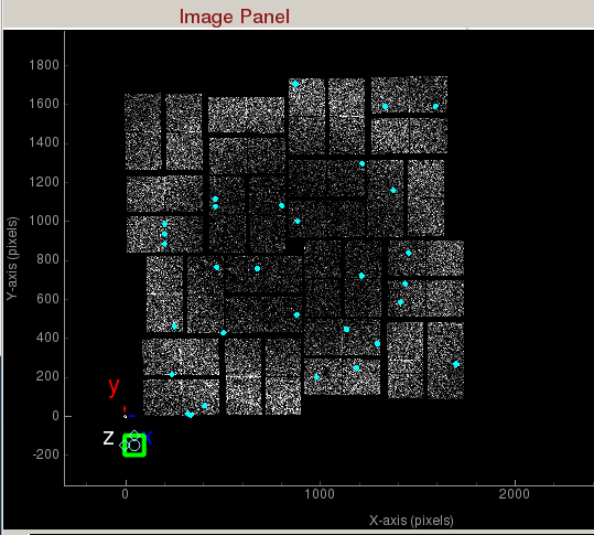
Peaks found are shown in cyan.Hit Finder
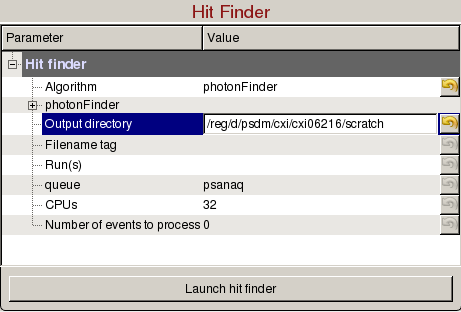
Hit Finder panel is used to tune hit finding parameters for detector images without peaks, and launch hit finding jobs on the computing cluster:
- Algorithm: Select the hit finding algorithm.
- photonFinder: Counts the number of pixels above ADU per photon.
- Output directory: Directory where the output hdf5 will be saved. The name of the file will be <experiment name>_<4 digit run number>.cxi, (e.g. cxi06216_0022.h5).
- Run(s): Comma separated list of run numbers to submit to the cluster, or colon for a range of runs, (e.g. 1,4:6,9 --> runs 1, 4, 5, 6, 9).
- queue: Name of the queue to use. You are only allowed to run from the hiprioq's during your experiment, because jobs on the hiprioq will suspend other running jobs in the same queue.
- CPUs: Number of CPUs to use per run.
- Number of events to process: Number of events to process. The default value of zero means process all the events in the run. Setting it to 1000 will process only the first 1000 events.
- Launch hit finder: Submit hit finding jobs to the cluster. It will be launched with the hit finding parameters and the mask (if defined).
- Algorithm: Select the hit finding algorithm.
Indexing
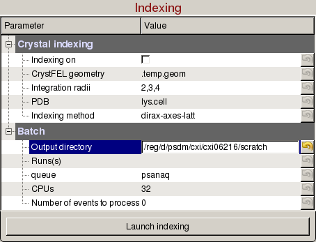
Indexing panel is used to tune indexing parameters for crystal diffraction patterns, and launch indexing jobs on the computing cluster:
- Indexing on: Check to turn on indexing results. Based on the peaks found in the peak finder panel, it will display peaks used to determine the orientation and unit cell parameters of the crystal. A big X means indexing failed.
- CrystFEL geometry: Full path of the geometry file used to index the crystal. Changing the detector distance in the Diffraction Geometry panel will update this geometry file.
- Integration radii: Inner circle is used for peak integration and outer ring is used to estimate the background level.
- PDB: Full path of the PDB file used to index the crystal (Optional).
- Indexing method: Comma separated list of indexing methods to try in the order of priority.
- Output directory: Directory where the output hdf5 will be saved. The name of the file will be <experiment name>_<4 digit run number>.cxi, (e.g. cxi06216_0022.h5).
- Run(s): Comma separated list of run numbers to submit to the cluster, or colon for a range of runs, (e.g. 1,4:6,9 --> runs 1, 4, 5, 6, 9).
- queue: Name of the queue to use. You are only allowed to run from the hiprioq's during your experiment, because jobs on the hiprioq will suspend other running jobs in the same queue.
- CPUs: Number of CPUs to use per run.
- Number of events to process: Number of events to process. The default value of zero means process all the events in the run. Setting it to 1000 will process only the first 1000 events.
- Launch indexing: Submit indexing jobs to the cluster. Turbo indexing will be used by splitting the run(s) into chunks, then the results will be merged into one stream file per run.
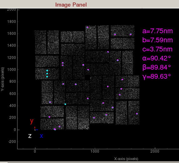
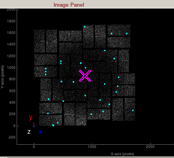
Indexed peaks are shown in magenta. Peaks found are shown in cyan. Each indexed peak are represented by the integration rings. The unit cell parameters are displayed on the side. A failed indexing result will be displayed as a big X.Mask Panel
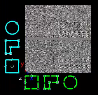
Mask Panel is used to generate masks on the assembled detector:- Use user-defined mask: Check to use user-defined mask. Three cyan Mask generators will appear left of the coordinate marker. User-defined masked pixels will show up as blue. Polygon mask generator is in the shape of the letter "P". You can add vertices by left clicking on an edge. You can remove a vertex by right clicking on a vertex and choosing "Remove handle".
- Masking mode:
- Off: Do not create mask.
- Toggle: Unmask masked areas under the ROI and mask unmasked areas under the ROI.
- Mask: Mask area under the ROI.
- Unmask: Unmask area under the ROI.
- Masking mode:
- Use jet streak mask: Check to turn on jet streak mask. Jet streak mask is shown as red.
- maximum streak length: Maximum jet streak length from end-to-end in pixels.
- sigma: Number of standard deviations away from mean to set the threshold.
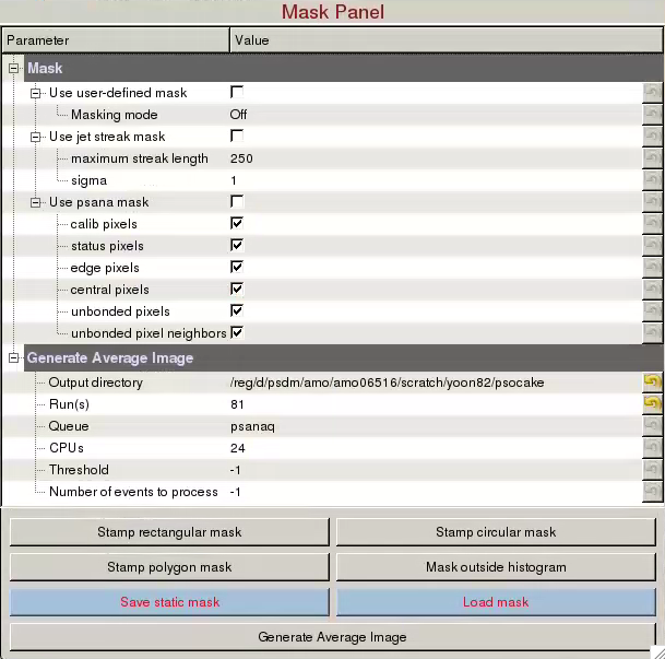
- Use psana mask: Check to turn on psana mask. Psana mask is shown as green.
- calib pixels: run-number-dependent user-defined masks deployed to the experiment's calibration directory.
- status pixels: bad pixels as determined from calibman dark-run analysis.
- edge pixels: edges of ASICS.
- central pixels: for a CSPAD the center rows of pixels of a 2x1 ASIC. which are larger than the other pixels.
- unbonded pixels: unbonded pixels.
- unbonded pixel neighbors: the 4 nearest neighbors of unbonded pixels.
- mask rectangular ROI:
- mask circular ROI:
- Save user-defined mask:
- Load user-defined mask:
Generate Average Image is used to generate average (mean,max,std,sum) images of the run:
- Output directory: Directory where the output numpy images will be saved. The name of the file will be <experiment name>_<4 digit run number>_<detName>_<type>.npy, (e.g. cxi06216_0022_mean.npy).
- Run(s): Comma separated list of run numbers to submit to the cluster, or colon for a range of runs, (e.g. 1,4:6,9 --> runs 1, 4, 5, 6, 9).
- queue: Name of the queue to use. You are only allowed to run from the hiprioq's during your experiment, because jobs on the hiprioq will suspend other running jobs in the same queue.
- CPUs: Number of CPUs to use per run.
- Threshold: ADU threshold on each image before averaging. The default value of -1 means do not threshold.
- Number of events to process: Number of events to process. The default value of -1 means process all the events in the run. Setting it to 1000 will process only the first 1000 events.
- Generate Average Image button: Submit averaging job to the cluster.
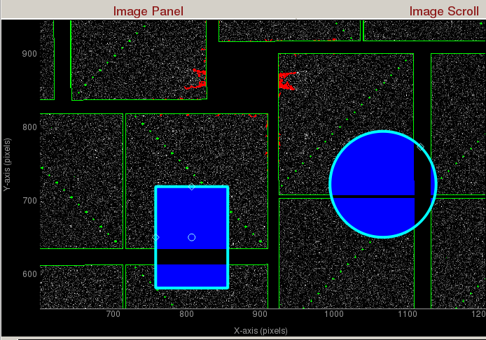
Zoomed in display of a CsPad detector. User-defined masks are shown as blue. Jet streaks are shown as red. Psana mask is shown as green.- Use user-defined mask: Check to use user-defined mask. Three cyan Mask generators will appear left of the coordinate marker. User-defined masked pixels will show up as blue. Polygon mask generator is in the shape of the letter "P". You can add vertices by left clicking on an edge. You can remove a vertex by right clicking on a vertex and choosing "Remove handle".
Overview
Content Tools