Validating ICMP ping measurements against TCP nping measurements

Introduction

There are several articles in the literature that warn against using ping/ICMP measurements of RTT compared to TCP and UDP measurements. See for example:

The concerns are that ICMP/ping RTT measurements are not representative of TCP RTTs since both the ISPs and the end-node sites de-priortitize ICMP compared to TCP and UDP based applications.

In 1998 we compared the round trip times (RTT) and losses measured by ping with those measured between sending the SYN packet for a TCP stream and receiving the ACK back. We found that the distributions agreed well, e.g. the median and average RTTs and losses agreed well (well within the Inter Quartile Range) of the distributions.

Since then there may have been increased de-prioritizing which could increase the differences in the two types of measurements, so we decided to re-evaluate the differences.

It would be good to quantitatively understand these differences and understand how they manifest themselves (e.g. region of world for targets, ipv4 and ipv6).

A project to quantitatively compare TCP and ICMP RTTs and losses would be to use hping3 (does not support ipv6) or nping (supports ipv6) to measure TCP RTTs and losses to multiple web servers (port 80) already pinged by PingER and compare them to those of similar ICMP. measurements (made from the same measurement agent (MA) at similar times)

For example we could use the command:

486cottrell@pinger:~$sudo nping -p 80 -c 2 -6 --tcp-connect 2001:da8:270:2018:f816:3eff:fef3:bd3
Starting Nping 0.5.51 ( http://nmap.org/nping ) at 2018-01-13 15:21 PST
SENT (0.0021s) Starting TCP Handshake > 2001:da8:270:2018:f816:3eff:fef3:bd3:80
RECV (0.1679s) Handshake with 2001:da8:270:2018:f816:3eff:fef3:bd3:80 completed
SENT (1.0041s) Starting TCP Handshake > 2001:da8:270:2018:f816:3eff:fef3:bd3:80
RECV (1.1692s) Handshake with 2001:da8:270:2018:f816:3eff:fef3:bd3:80 completed
Max rtt: 165.789ms | Min rtt: 165.073ms | Avg rtt: 165.431ms
TCP connection attempts: 2 | Successful connections: 2 | Failed: 0 (0.00%)
Tx time: 1.00329s | Tx bytes/s: 159.48 | Tx pkts/s: 1.99
Rx time: 1.16836s | Rx bytes/s: 68.47 | Rx pkts/s: 1.71
Nping done: 1 IP address pinged in 1.17 seconds

Together with this, we could use the list of PingER perfSONAR hosts that respond to pings. Note that sometimes pings are blocked to a host but TCP port 80 packets work, e.g. adl-a-ext1.aarnet.net.au (202.158.195.68).

Project

We wrote a script ping-vs-tcp.pl* for analyzing the PingER nodes, and another ping-vs-tcp-ps.pl for analyzing perfSONAR nodes. For more information see here.

Usage:   ping-vs-tcp.pl [opts]
        Opts:
        --help     print this USAGE information
        --debug    debug_level (default=0)
        --prot    protocol (6 or '') (default '')
        --port     application port (default = 80)
        --count    count of pings or npings to be sent (default = 10)
Function:
  Ping the host provided in %NODE_DETAILS
  For each host it gets the IP address either from NODE_DETAILS (IPv4)
  or using the dig command (IPv6).
  It then Pings and npings the host and gathers the min, average, maximum
  RTTs and losses and reports them to STDOUT, together with a time stamp
  and host information  such as name, IP address, contry, region etc.
Externals:
  Requires nping (requires root/sudo privs), dig
Input:
  It gets information on the PingER hosts from %NODE_DETAILS using:
  wget to get the required file from http://www-iepm.slac.stanford.edu/pinger/pingerworld/slaconly-nodes.cf.
  The required file is saved in tmp with a unique name /tmp/nodes-9020.cf
  (where the number is based on the process number).
Examples:
 ping-vs-tcp.pl
 ping-vs-tcp.pl --prot 6 --port 22 --count 10 | tee pg-v4-nd.txt
 ping-vs-tcp.pl --help
Hint:
 To turn the output into a real csv file do something like:
 grep warning pg-v4-db.txt  > pg-v4-nd.csv
Version=0.4, 1/28/2018, Cottrell

The output is in comma separated value format and is exported to Excel (one file for IPv4, one for IPv6) where it is analyzed to look at the histograms of Avg(ping-rtt) and Avg(nping-rtt) etc. The script was run from a host (pinger.slac.stanford.edu) located at SLAC in Northern California in the San Francisco Bay Area. It was run multiple times to ensure the behavior was not dependent on time of day or day of week etc. To ensure the selected target hosts were not unique in some respect we also obtained a list of target hosts from the perfSONAR project and repeated the analysis for them. Finally, to ensure there was not something unique about making the measurements from SLAC, we repeated the measurements to the same sets of targets from MAs in China, Malaysia, and Thailand. For more information on the

IPv4 measurements

For the IPv4 data measurements using the list of PingER hosts, for the IPv4 hosts the script ran for about 6 hours and 45 minutes. The distribution histograms shown below show that the agreement between ping and nping average RTT is good:

PIngER targets from SLAC:

There are 728 PingER hosts responding to both ping and nping on port 80 (there are about 270 responding to port 22), 50% have Average(RTTs) for ping and nping within 2.15ms of one another. The hosts are in 160 different countries with China having the most hosts with 195, followed by the United States with 52, Indonesia with 37, Malaysia with 27 and Pakistan with 13. In terms of regions the top region is East Asia with 206 hosts, 101 from Africa, 63 from Europe and 58 from North America (Canada and the United States). There are 593 host that have 'www' in the name. The range of average ping RTTs is from 0.327ms to 377ms. The range of nping RTTs is from 2.3ms to 387ms.
The Frequency histograms of average ping and average nping RTTS are shown below (Excel spreadsheet is here)

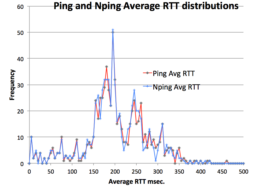It is seen that there is little difference in the two distributions. We thus compare the Cumulative Distribution Frequencies (CDF) by plotting their differences, note this is a step towards using the Kolmogorov–Smirnov (K-S) nonparametric test of the equality of continuous, one-dimensional probability distributions and yields a maximum difference (supremum) of 3.18% at 255 msec. K-S indicates that the probability of rejecting the null hypothesis (the null hypothesis says there is no relationship between the two measured phenomena) is very high.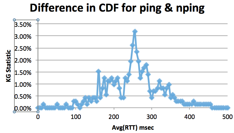

To exemplify the differences in the RTTs measured by ping and nping we show the frequency distribution of the differences in the two Average RTTs. The histogram of the differences in the ping and nping averages RTTs is shown below.

Another way of looking at the data is to consider the relative differences, i.e. (Avg(ping_RTT)-Avg(nping_RTT)/(0.5(Avg(ping_rtt)+Avg(nping_RTT)), this gives the distribution below that shows the IQR of the averge difference is ~ 1.2%. If one looks at the hosts that have relative differences of > 22% or less than -22% (about 2% of the hosts), we find most are from China or have low RTTs (< 4 msec).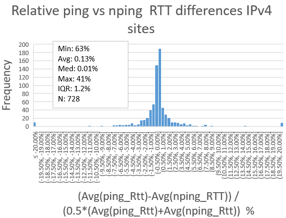

perfSONAR targets from SLAC

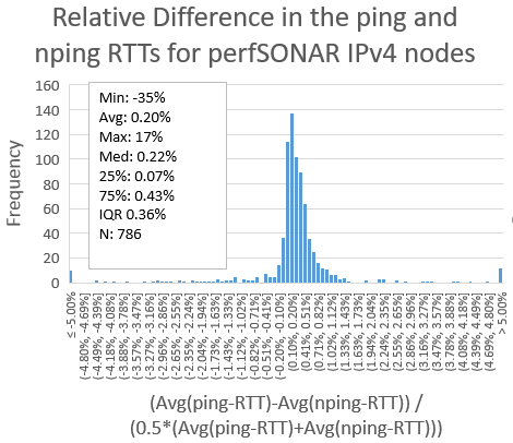
There are 786 perfSONAR target hosts that respond to both ping and nping IPv4 measurements. There are 317 in Canada and the US, 134 in 29 countries in Europe, 18 in E. Asia (all in Korea), 14 in Russia, 12 in Africa(Senega(2), Nigeria(1), Uganda(3), Niger(1), Ghana(4), Togo(1)) and 4 in each of S. Asia (3 in India and 1 in Pakistan) and Latin America (Brazil, Ecuador and Puerto Rica(2)). The regions for the other hosts are not identied in the perfSONAR database.

Histograms of the frequency distributions are shown below, the Excel spread sheet is here.:

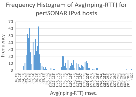IPv6 measurements

PingER hosts seen from SLAC MA

There were about 35 IPv6 hosts in the PingER list

PingER targets: 50% of the 36 hosts measured have average(RTTs) within 0.26ms of oneanother).

Again the relative ping vs nping differences for IPv6 is shown below and shows an IQR of the relative average difference is 0.45%:

perfSONAR targets

From the perfSONAR JSON configuration file we found 154 hosts that have IPv6 addresses (see spreadsheet). Of these (using the perl script bin/ping-vs-tcp-ps-sq.pl --conf ps-v6-sq.cf | tee ps-v6-sq.txt, it ran for about 45 minutes) we found 6 hosts that did not respond to ping6 and 50 for which we were was unable to get the information from nping. This yielded 98 IPv6 capable perfSONAR nodes that respond to ping6 and nping. Of these 53 are in N. America (Canada and the U.S.), 30 in Europe (13 in the United Kingdom), 4 in Russia, and 1 each in Africa (Uganda) and Costa Rica. The spreadsheet is here.

perfSONAR hosts seen from Chinese MA

The MA was at a CERNET host in Beijing. The spreadsheet of the results is here.

Histogram of difference in Avg(ping-RTT)-Avg(nping-RTT) for IPv6 measured from China
Histogram of the relative difference between ping and nping RTTs measured from China
Cumulative Distribution Frequency of the Avg(ping-RTT) and Avg(nping-RTT) with the differences.

The maximum(abs(Difference))=D is 0.031. We use the Kolmogorov Smirnov two sample test. for the number of observations (N), c(alpha) > D/sqrt(2N/N*N), where alpha indicates that the probability of rejecting the null hypothesis (the null hypothesis says there is no relationship between the two measured phenomena) is 85%.