NOTE: Please consider the following notes as more of a brain dump instead of a well thought out document.
Update 06/07/2018
- Looked into Traffic Differentiation - Rate Limiting vs. Traffic Prioritization (QoS)
- Conclusions:
- Min RTT essentially reflects fixed delay, while average RTT subsumes variations and path load
- TCP Segment drops manifest as large increases in delay
- QoS can be implemented in at least two ways:
- When priorities are implemented, ICMP packets will only be dropped if ICMP quota is full and link is congested, otherwise ICMP traffic is allowed to go beyond quota
- When rate-limits are implemented, ICMP packets will be dropped when ICMP quota is met, even if links are not congested
- Path loads dictate latency estimates: With weighted QoS implementations, loaded links depress ICMP
- Min RTT essentially reflects fixed delay, while average RTT subsumes variations and path load
- Found relevant papers and technical reports. The intent here is to understand the components of latency to help with the evaluation.
Y. Zhang, N. Duffield, V. Paxson, S. Shenker, On the Constancy of Internet Path Properties, in ACM SIGCOMM Internet Measurement Workshop 2001
A. Acharya, J. Saltz, A Study of Internet Round-Trip Delay, Univ of Maryland, Tech Rep. CS-TR-3736
M. Allman, V. Paxson, On Estimating End-to-End Network Path Properties, in ACM SIGCOMM 1999
V. Paxson, G. Almes, J. Mathis, Framework for IP Performance Metrics
- Setup NeuBot and experimented with tests but wasn't able to find useful examples of traffic differentiation (see https://www.measurementlab.net/tests/)
- Skimmed Glasnost to understand traffic shaping (see http://broadband.mpi-sws.org/transparency/glasnost.php and https://github.com/marcelscode/glasnost)
- [Not Relevant] Miscellaneous notes on ICMP Traceroutes, MPLS tunneling & ICMP (see http://cluepon.net/ras/traceroute.pdf), Measuring Performance
What are we investigating?
We've come across comments that under certain conditions ICMP ping may not provide reliable results. This may be due to several reasons, including how ICMP traffic is treated when flowing through the network.
Therefore, we want to study: if there are cases where ICMP ping provides different latency results than those provided by TCP based tools, e.g., TCP ping (https://nmap.org/nping/).
From here onwards, I will refer to ICMP ping measurements as ping and TCP ping measurements as nping.
Side note: It may also be argued that TCP ping is a better representative of application experience as TCP ping's traffic will face the same issues as that of the application (e.g., packet reordering and segregation). Therefore, it may be relevant to consider other tools such as owamp (http://software.internet2.edu/owamp/).
What to measure and how to analyze?
It is apparent that the metric to measure is "Latency". Les has put together a script that collects latency measurements using ICMP ping and TCP nping from a specific node. (For example, we've collected results from nodes at SLAC and VT.) This script provides the minimum, maximum, and average RTT measurements using both ping and nping. See document (https://confluence.slac.stanford.edu/display/IEPM/Validating+ICMP+ping+measurements+against+TCP+nping+measurements) for further details.
Given the wide coverage of PingER, we are in an ideal position to collect latency measurements from across the world.
Given the question that we are trying to answer (which in other words may be: how accurate is ping in comparison to nping), we would have to compare ping to nping measurements between pairs of nodes. For example, we would analyze the ping vs nping latency between SLAC and CERN, while measurements between SLAC and CALTECH will be treated separately.
It would not make sense to combine ping measurements from SLAC to CERN and SLAC to CALTECH as a single "ping" set. Similarly, we wouldn't combine nping measurements from SLAC to CERN and SLAC to CALTECH into a single "nping" set. Let us try a proof by contradiction: Say we were to combine ping measurements to all remote sites in a single "ping" data set and similary all "nping" measurements in another data set. Assume that the SLAC to CALTECH ping measurements are of 80ms (in the first set) and the nping measurements are of 85ms (in the second set). How are we to tell when comparing CDFs of the two sets that the ping (80ms) is being compared to nping (85ms) datum? What if the SLAC to CALTECH ping measurement goes in the 23% bucket, and the nping measurement goes in the 25% bucket. Therefore, it has to be a one-to-one comparison i.e., we would compare the ping and nping measurements between a pair of sites.
One might argue the validity of round-trip times (RTTs) in case of asymmetric routes. We will have to answer this issue when writing a paper, which we can do by demonstrating symmetric routes between test cases by sharing traceroutes between (to and from) the peers. For the time being we can ignore test-cases where there are asymmetric routes.
Components of latency
Before we delve into the analysis, it would be instructive to understand what constitutes latency. Here are some URLs that describe the breakdown.
https://www.o3bnetworks.com/wp-content/uploads/2015/02/white-paper_latency-matters.pdf
https://hpbn.co/primer-on-latency-and-bandwidth/
For the sake of our study, I would break down the one-way latency into the following components. Assuming symmetric routes, we can simply double the latency to estimate RTT.
- Time taken for the packets to traverse down the stack (from the application, via sockets API, network, link. I imagine ICMP uses RAW sockets, while nping would regular TCP sockets. It would be prudent to confirm by looking at the code.)
- Time taken for the frames to reach the recipient (includes transmission delay, propogation delay, and queueing delay)
- Time taken for the packets to traverse up the stack
What would introduce and difference in the latencies?
When we consider the breakdown above, it appears that factors causing different results would be:
- Additional delay in processing TCP segments (at the transport layer) vs raw IP packets
- Difference in delay because ICMP traffic was treated differently as it flowed through the network
We would expect that the above aspects are the only two aspects that would create a difference. We will have to assume the following though:
- The routes do not change during the experiments (i.e., the same routes were used for both flows)
- The routes were symmetric
- Similar volume and types of cross traffic was experienced by the packets
We would need some instrumentation to measure the amount of time it takes for an ICMP packet and a TCP packet to be processed by the stack. Alternatively, we may also refer to recent research that may have looked at such measurements. For example, we could use strace to measure time taken by socket API / system calls. (strace has a -T option for timestamps.) There are network stack implementations that include instrumentation (I can't seem to recall the names. I'll google for them later.)
Preliminary analysis
Based on the above discussion and assumptions, I've tried to understand the measurements. If we change our approach, we'll have to revise our analysis too.
Experiment setup
I made a slight modification to Les' script, in that I wrapped the experiment in a 1-50 iterations loop. This would provide us repeated experiemnts. I will attach the modified code to this page. Please see download links at the bottom.
The fifty measurements allow us to have a sufficiently large sample size. Considering the central limit theorem, we can use the samples to test for normality. Note that Les' scripts takes an average of the measurements. We then repeat these experiments 50 times. Therefore, we would expect a normal distribution and therefore can use ANOVA. For now, Les' script uses 10 measurements. Increasing the count to 30 will guarantee that we always have a normal distribution.
In some cases, we do see outliers. Typically, in papers we would be expected to explain the outliers. However, as we do not control the environment, I would attribute the outliers to variation due to cross traffic or factors beyond our control. As we have an abundance of data, for now we can simply ignore pairs with large number of outliers. At a later stage, we can come back to understand why we see the outliers.
Analysis using One-way ANOVA and Kolmogorov-Smirnov two-sample tests
ANOVA assumes: a) independence, b) normality of residuals, and c) homogeniety of variances.
We can confidently assume independence as each latency test has no bearing on the next. The first ping may take slightly longer than the following as forwarding tables may need to be updated, or arp tables may been to be populated. However, subsequent tests would be completely indepedent. We can address this aspect by increasing the number of experiments from 30 to 31 (or 10 to 11), to cater to this requirement. For now, I have not modified the script in this regard.
The assumption is that "distributions of the populations from which the samples are selected are normal." We can test for normality using the Shapiro-Wilks test or by eye-balling qqplots.
The assumption is that the variance of samples from the population are the same. We can test for this assumption using the bartlett test. Note that if the aspects discussed in Section 3 remain the same, we know that the variances will remain the same.
If for some reason, the assumptions are violated, then we can simply use the Kolmogorov-Smirnov two-sample test.
For all the cases the null hypothesis is: there is no difference between icmp ping and tcp ping samples.
Below are few examples. Please see the download links at the bottom to for more examples. The whiskers in the boxplots represent 95% confidence intervals, while the horizontal line in the center is the median. The bottom and top horizontal lines are the first and third quartiles. (Perhaps, we should change the whiskers to reflect standard deviation.)
mit.edu:
Two-sample Kolmogorov-Smirnov test
data: sub_df$ping_avg and sub_df$nping_avg
D = 0.28, p-value = 0.03968
alternative hypothesis: two-sided

Shapiro-Wilk normality test
data: sub_df$ping_avg
W = 0.97335, p-value = 0.315

Shapiro-Wilk normality test
data: sub_df$nping_avg
W = 0.98432, p-value = 0.7418
[1] "ANOVA Summary"
Df Sum Sq Mean Sq F value Pr(>F)
tool 1 5.48 5.481 8.218 0.00508 **
Residuals 98 65.35 0.667
---
Signif. codes: 0 ‘***’ 0.001 ‘**’ 0.01 ‘*’ 0.05 ‘.’ 0.1 ‘ ’ 1
| mit.edu: qqplot for ping | mit.edu: qqplot for nping | mit.edu: boxplot |
|---|---|---|
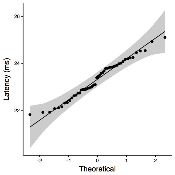 | 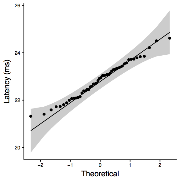 | 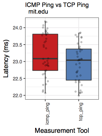 |
Observation: KS test tells us that we cannot reject the null hypothesis (that they are the same). Note that the p-value is marginal (i.e., close to 0.05).
www.globalone.com.br:
Two-sample Kolmogorov-Smirnov test
data: sub_df$ping_avg and sub_df$nping_avg
D = 0.68, p-value = 2.668e-11
alternative hypothesis: two-sided

Shapiro-Wilk normality test
data: sub_df$ping_avg
W = 0.84507, p-value = 1.141e-05

Shapiro-Wilk normality test
data: sub_df$nping_avg
W = 0.96575, p-value = 0.1547
[1] "ANOVA Summary"
Df Sum Sq Mean Sq F value Pr(>F)
tool 1 547.9 547.9 71.71 2.52e-13 ***
Residuals 98 748.8 7.6
---
Signif. codes: 0 ‘***’ 0.001 ‘**’ 0.01 ‘*’ 0.05 ‘.’ 0.1 ‘ ’ 1
| www.globalone.com.br: qqplot for ping | www.globalone.com.br: qqplot for nping | www.globalone.com.br: boxplot |
|---|---|---|
 | 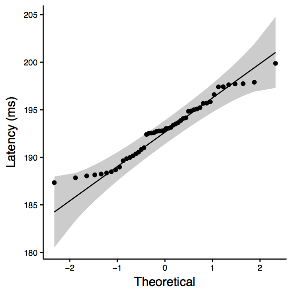 | 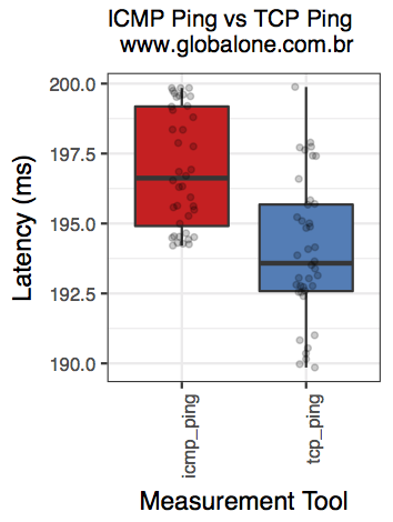 |
Observation: KS test tells is that we can reject the null hypothesis (that there is not enough evidence to confim that they are the same.)
www.git.edu.cn:
Two-sample Kolmogorov-Smirnov test
data: sub_df$ping_avg and sub_df$nping_avg
D = 0.52083, p-value = 2.667e-06
alternative hypothesis: two-sided

Shapiro-Wilk normality test
data: sub_df$ping_avg
W = 0.54406, p-value = 5.471e-11

Shapiro-Wilk normality test
data: sub_df$nping_avg
W = 0.66366, p-value = 3.198e-09
[1] "ANOVA Summary"
Df Sum Sq Mean Sq F value Pr(>F)
tool 1 30509 30509 12.74 0.000566 ***
Residuals 94 225081 2394
---
Signif. codes: 0 ‘***’ 0.001 ‘**’ 0.01 ‘*’ 0.05 ‘.’ 0.1 ‘ ’ 1
| www.git.edu.cn: qqplot for ping | www.git.edu.cn: qqplot for nping | www.git.edu.cn: boxplot |
|---|---|---|
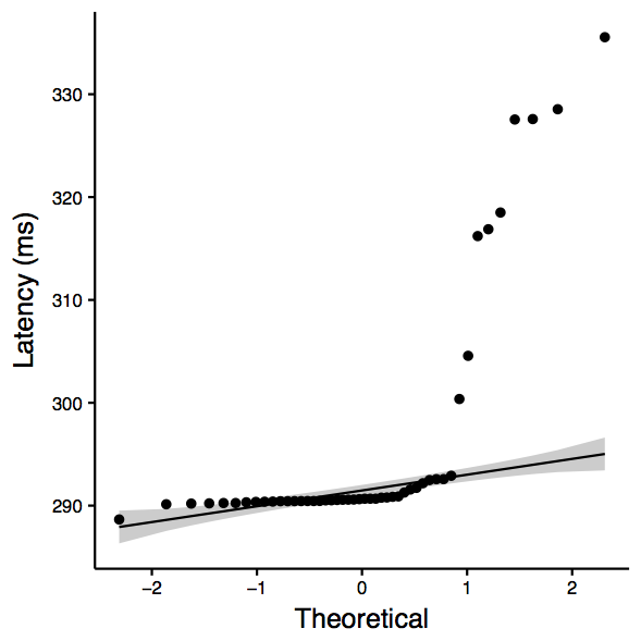 | 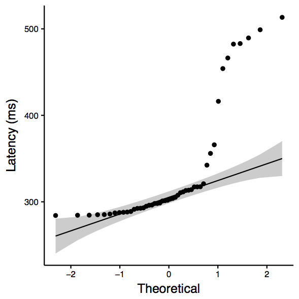 | 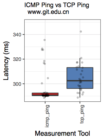 |
Observation: Although the QQplots show outliers, the shapiro test confirms normality. Therefore, we consider ANOVA, which is significant and therefore we can reject the null hypothesis (that there is not enough evidence to confim that they are the same.)
Region-wise breakdown
The results also includes region-wise breakdown. Download the "processed output" archive from the links below to see all the region plots.
| North America | Balkans |
|---|---|
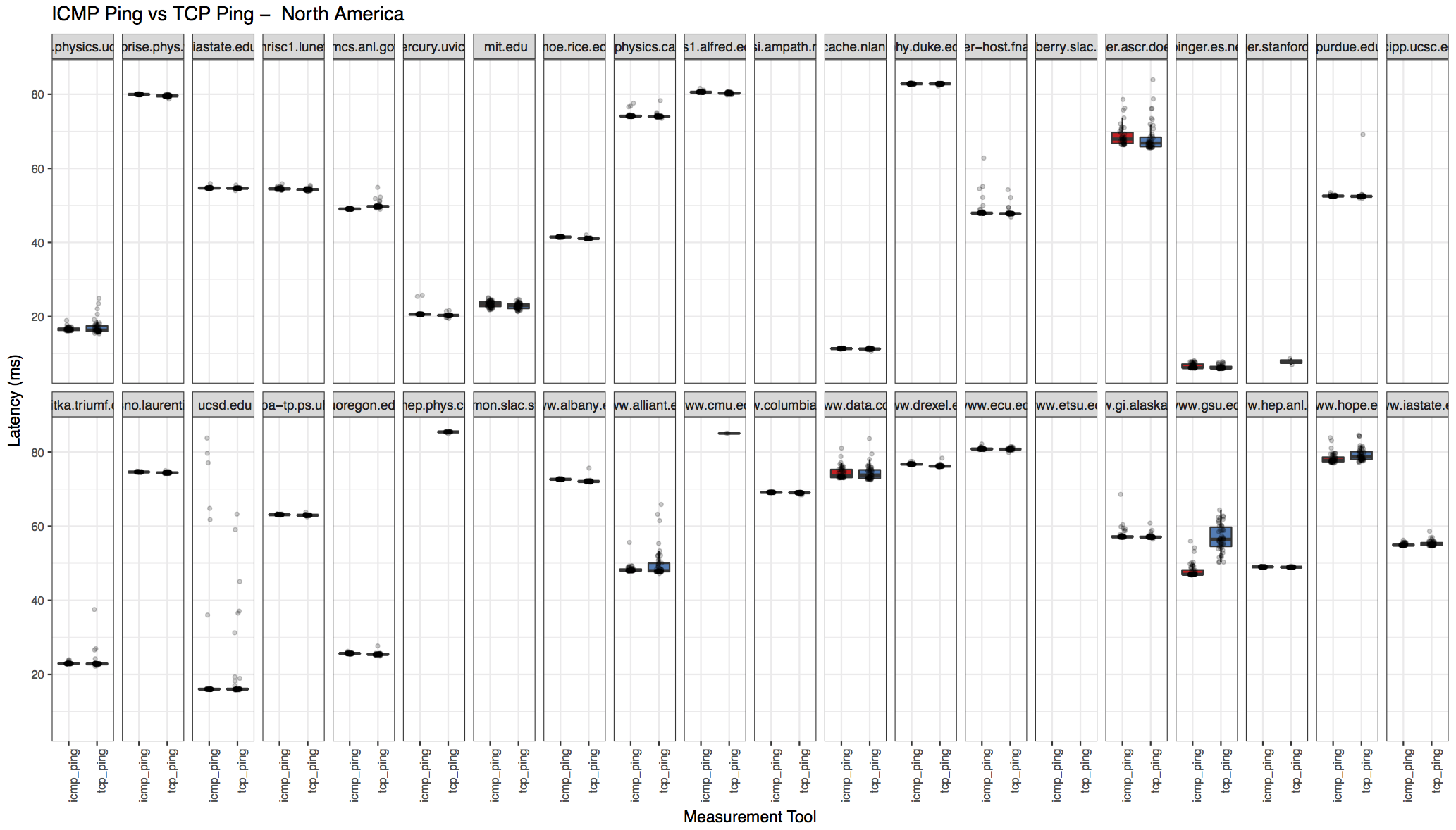 | 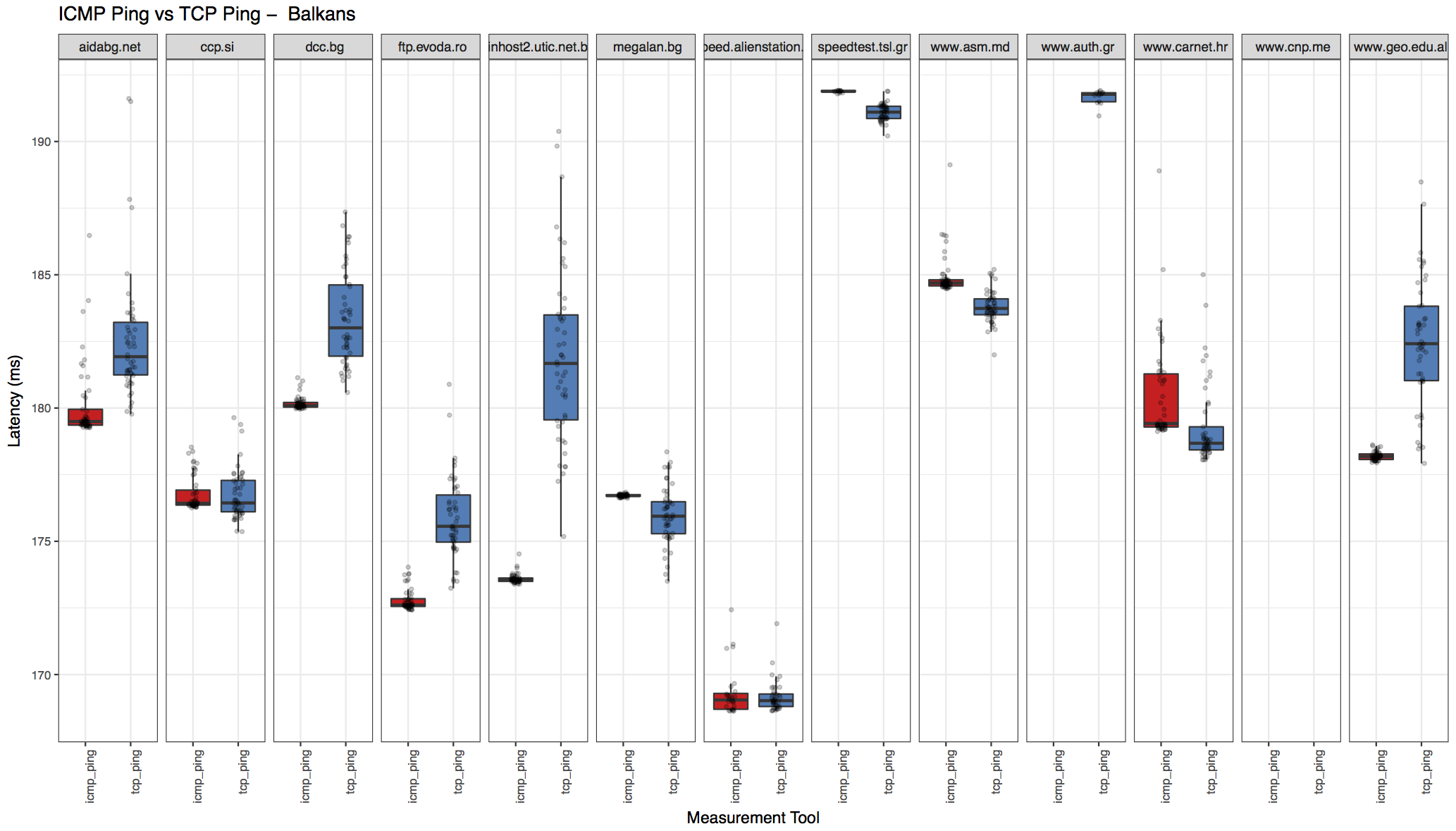 |
Analysis Script & Download Links
Once the logs from Les' script are available, they may be passed onto the analyze.r script for processing and generating output. I am attaching an example of processed output here.
Here are the download links:
- ping-vs-tcp.pl
- analyze.r
- partial input for analysis (2018-03-02-slac-v4-uk) (i.e., output of ping-vs-tcp.pl)
- processed output and associated files (2018-03-02-slac-v4-uk)
Requirements for running analysis script
You would need to install R and the necessary libraries. Once R is installed, you may install the libraries as follows:
# R Commands:
install.packages("optparse")
install.packages("dplyr")
install.packages("ggpubr")
install.packages("tidyr")
install.packages("ggplot2")
To process input, simply run the analyze script from the console. (Alternatively, you can use the contents of the script to run within R.):
# query for help
$ Rscript analyze.r -h
	-i CHARACTER, --inputfile=CHARACTER
	path to input file (e.g., 2018-02-21-pg-v4-uk-vt.log)


# example run
$ ./analyze.r -i 2018-03-02-slac-v4-uk.log
Data Collection
$ sudo ./ping-vs-tcp.pl --prot 4 --port 80 --count 3 | tee 2018-03-02-ps-v4-uk.log
$ tail -20 2018-03-02-ps-v4-uk.log
$ tmux ls
1: 1 windows (created Tue Mar 27 11:32:10 2018) [156x85]
default: 1 windows (created Tue Mar 27 11:32:10 2018) [80x24]

$ tmux a -t 1