"Data analysis == Piece of cake"
Sections in this tutorial
It is always a good idea for the people doing analysis to look at their detector images and be able to probe intensity values. Given that a typical LCLS experiment has millions of snapshots to choose from, it is also critical that you can quickly select images of interest and set regions of interest using masks. By the end of this tutorial, you will be able to browse images, jump to images of interest, generate masks, find peaks in your images, index crystal diffraction patterns, and change the x,y,z positions of your detector.
Citation for psocake (and other psana-based programs):
@Article{Thayer2017,
author="Thayer, J. and Damiani, D. and Ford, C. and Dubrovin, M. and Gaponenko, I. and O'Grady, C. P. and Kroeger, W. and Pines, J. and Lane, T. J. and Salnikov, A. and Schneider, D. and Tookey, T. and Weaver, M. and Yoon, C. H. and Perazzo, A.",
title="Data systems for the Linac coherent light source",
journal="Advanced Structural and Chemical Imaging",
year="2017", month="Jan", day="14", volume="3", number="1", pages="3", issn="2198-0926",
doi="10.1186/s40679-016-0037-7", url="https://doi.org/10.1186/s40679-016-0037-7"}

@article{Damiani:zw5004,
author = "Damiani, D. and Dubrovin, M. and Gaponenko, I. and Kroeger, W. and Lane, T. J. and Mitra, A.
and O'Grady, C. P. and Salnikov, A. and Sanchez-Gonzalez, A. and Schneider, D. and Yoon, C. H.",
title = "{Linac Coherent Light Source data analysis using {it psana}}",
journal = "Journal of Applied Crystallography",
year = "2016", volume = "49", number = "2", pages = "672--679", month = "Apr",
doi = {10.1107/S1600576716004349}, url = {http://dx.doi.org/10.1107/S1600576716004349}, }
Please connect to psana machines via NoMachine for less lag in graphics. Instructions here: Remote Visualization
Starting psocake in SFX mode
If you are on a psana machine, set up your environment by adding these lines to your ~/.bashrc (or your start up script):
# PSOCAKE2 (Run 17 or older)
function psocake2 ()
{
    echo "Activating psocake py2"
    source /reg/g/psdm/etc/psconda.sh -py2
    source /reg/g/cfel/crystfel/crystfel-0.8.0/setup-sh # CrystFEL compatible version for psocake2
}

# PSOCAKE3 (Run 18 or newer)
function psocake3 ()
{
    echo "Activating psocake py3"
    source /reg/g/psdm/etc/psconda.sh
    source /reg/g/cfel/crystfel/crystfel-0.9.1/setup-sh # Crystfel compatible version for psocake3
}

# CCP4 (version may change)
source /reg/common/package/ccp4-7.1/bin/ccp4.setup-sh
# XDS
export PATH=/reg/common/package/XDS-INTEL64_Linux_x86_64:$PATH
Then source ~/.bashrc
For LCLS Run 18 or newer runs, call the psocake3 function by typing psocake3 in the terminal.
For older LCLS runs, use psocake2.
$ source ~/.bashrc
$ psocake3
Activating psocake py3
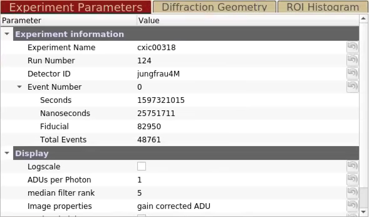
For this tutorial, we will look at experiment cxic00318, run 124, detector jungfrau4M, event 33.
1) There are four parameters required to uniquely identify an image at LCLS. Type the (1) experiment name, (2) run number, (3) detector name, and (4) event number in the Experiment Parameters panel.
2) You can specify the experiment parameters as command line arguments in psocake using the psana-style experiment run string. This is the recommended way of starting psocake:
$ psocake exp=cxic00318:run=124 -d jungfrau4M -m sfx
Or you can also use the -e and -r arguments for the experiment and the run number:
$ psocake -e cxic00318 -r 124 -d jungfrau4M -m sfx
Note: GUI widgets may not respond properly when the GUI is first displayed. Clicking on the terminal window or resizing the GUI will fix this.
During the experiment, you have access to Fast Feedback System which allows you to run psocake from Fast Feedback (FFB) nodes. To do this, append -a ffb. Note that only psffb has access to the data on FFB:
$ psocake -e cxic00318 -r 124 -d jungfrau4M -m sfx -a ffb
Note that available detector names will be printed on the terminal once you have typed in the experiment name and the run number.
#######################################
# Available area detectors:
# ('CxiDs1.0:Jungfrau.0', 'jungfrau4M', '')
#######################################
CxiDs1.0:Jungfrau.0 is the full detector name. jungfrau4M is the simpler DAQ alias. In most cases, Psocake can understand both naming conventions.
To check psocake version:
$ psocake --version
Don’t worry if you don’t remember these arguments. You can view argument options using --help:
$ psocake --help
Psocake should have generated directories and files in the experiment directory. At LCLS, all experiments are stored here: /reg/d/psdm/<instrument>/<experiment>. Let's take a moment and check out our directory structure. Either open a new terminal (Remember to 'ssh psana') or use the current terminal ('Ctrl+z' to suspend psocake that is running then 'bg' to run psocake in the background), type the following command:
$ ls /reg/d/psdm/cxi/cxic00318
calib  hdf5  results  scratch  stats  usrdaq  xtc
calib: This is where all psana calibration is stored. Detector geometry, pedestals, gain, common mode constants, and bad pixelmap.
xtc: This is where all your raw data is stored. XTC is an efficient format for storing large data which can be read using psana. Note you have 4 months to analyse your data before xtcs are moved off to tape.
scratch: This is where psocake saves all the files like .cxi and .stream. This directory is not backed up, so important files need to be backed up in /results.
results (or res): This is the results directory which is backed up on tape. After completing your analysis, your results/data should be moved here.
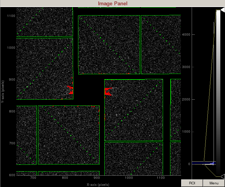
Browse images
Let's learn how to display images and read pixel values.
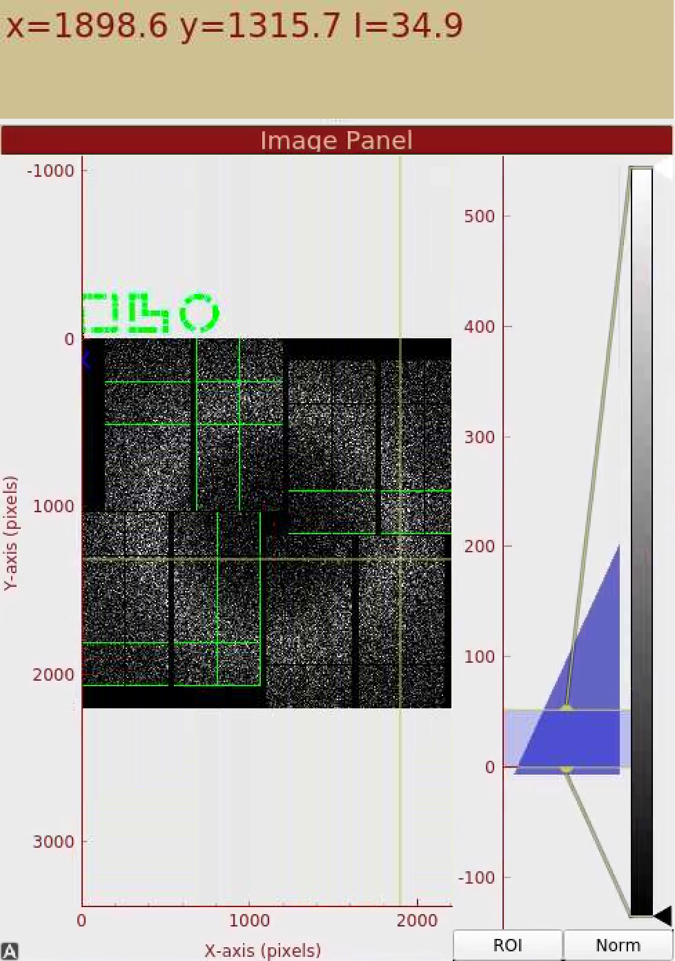
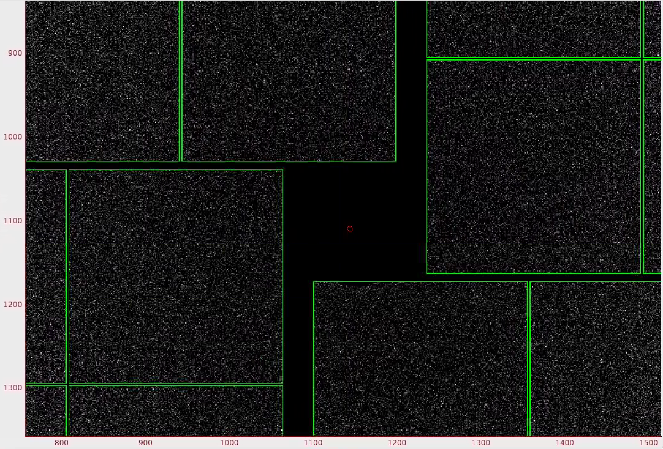
The Image Panel displays the gain-corrected image. The dynamic range for the display can be adjusted by dragging the two horizontal yellow bars on the intensity histogram on the right. By mousing over the detector pixels, the x,y position and pixel value are displayed above the panel.
The Experiment Parameters Panel shows which detector image is being displayed. You can type in an event number in the "Event Number" field to display the image.
There are also "Prev evt" and "Next evt" buttons to decrease and increase the event number, respectively. These are located in the lower right corner of the GUI. If you have already ran the peak finder for this run, you will see a blue scatter plot of the number of peaks found for each event. The markers on the scatter plot are clickable and will update the event number and the detector image.
Mask making
In this section, you will learn how to mask out pixels that should not be used for analysis (such as dead pixels and shadows), mask out the jet streak at the centre of the detector, and mask out the water ring (just for fun!). Masked out regions are ignored during peak finding and during Bragg spot integration.
Note: the Image Panel must be in the default "greyscale" colormap for the mask colors to display properly.
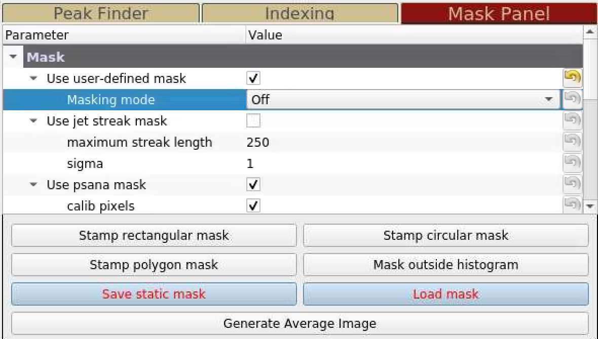
1) In the mask panel, "Use psana mask" checkbox is turned on by default.
This will mask out the following pixels that should not be used for analysis; calib, status, edge, central, unbonded pixels, unbonded pixel neighbor. Hovering over the checkboxes shows what these options mean. These masked pixels are shown as green on the image panel. You can selectively turn these on and off. Red circle indicates the detector centre.
2) To mask out jet streak near the centre of the detector, click on "Use streak mask".
This will mask out strong intensities originating from the liquid jet. The streak mask is dynamic, i.e. recalculated for each image.
3) Let's look at using the mask widgets.
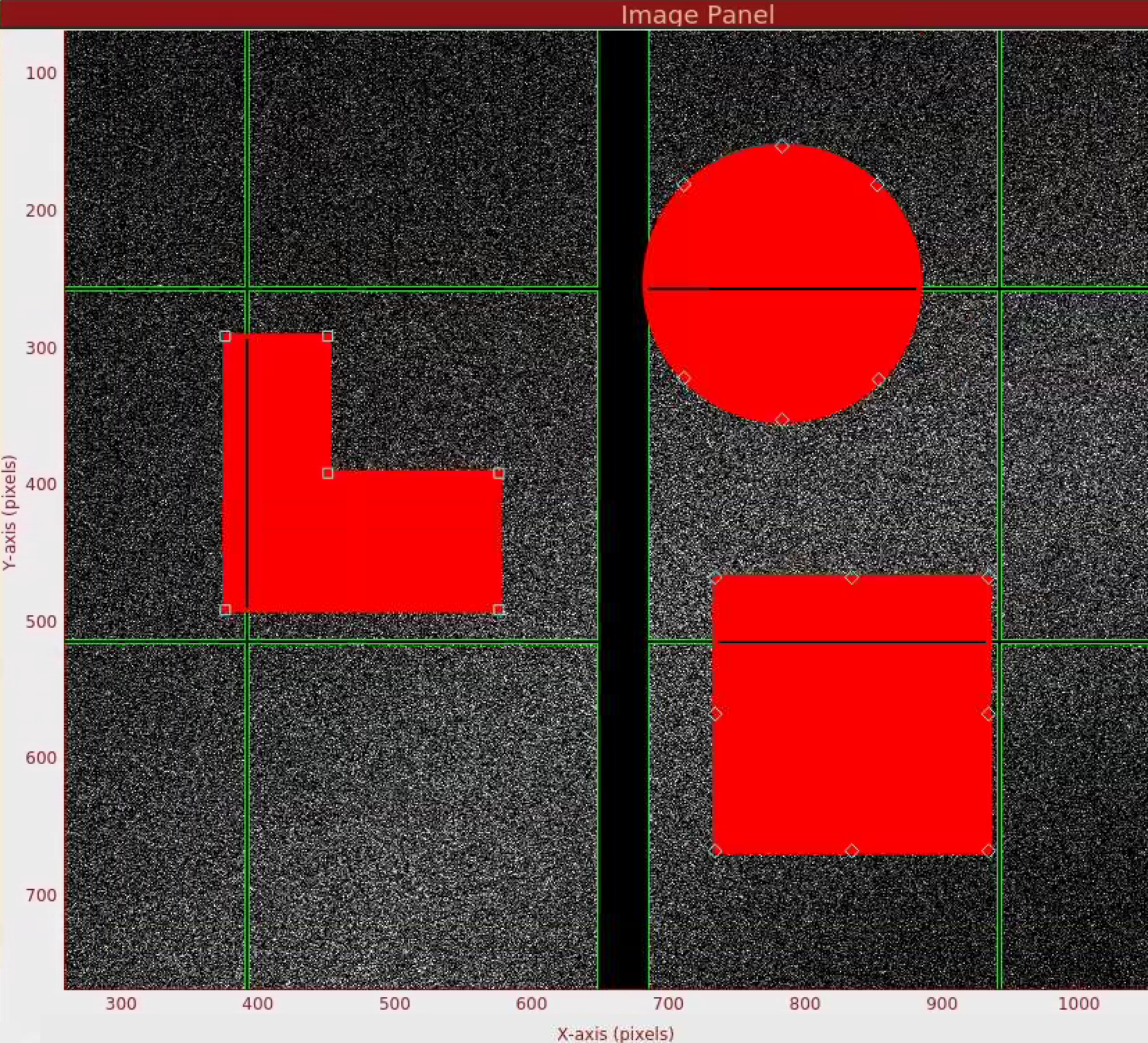
In the Mask Panel, turn on "Use user-defined mask". Select "Mask" in Masking mode. This will bring up a red rectangular, circle, and polygon mask widgets on the left of the detector image. You can drag a mask widget onto the detector by clicking and holding the mouse button inside a widget. There are diamond handles on these widgets which you can drag to resize. For the polygon widget, you can create additional handles (or corners) by a single click on the edge of the widget. Once positioned, use the "Stamp rectangular mask", "Stamp circular mask", and "Stamp polygon mask" buttons to create the mask. In this "Mask" mode, you can click on single pixels on the detector to make out single pixels. "Mask outside histogram" button will mask out pixels that are below the histogram low threshold and above the histogram high threshold.
To save the user-defined mask, click on "Save static mask" button on the mask panel which will save the mask in your designated psocake run folder. This will combine user-defined mask (red) and the psana mask (green) into a single mask. You should see the following message in the terminal:
Saving mask to /reg/d/psdm/cxi/cxic00318/scratch/<username>/psocake/r0124
*** deploy user-defined mask as mask.txt and mask.npy as DAQ shape ***
*** deploy user-defined mask as mask_natural_shape.npy as natural shape ***
Saving Cheetah static mask in:  /reg/d/psdm/cxi/cxic00318/scratch/<username>/psocake/r0124/staticMask.h5
mask.npy has the shape (8, 512, 1024) for this jungfrau4M detector. We refer to this shape as an unassembled 3D ndarray which can be used in psana python scripts.
mask.txt is in a 2D text format which is compatible with detector related files in the LCLS calibration folder.
You can load this mask in psocake by clicking the "Load mask" button and selecting mask.npy.
To delete the mask on the screen, select "Unmask" under Masking mode. Drag one of the red mask widgets over the detector and click "Stamp circular mask".
4) To make a donut mask over the water ring, turn on "Use user-defined mask". Select "Toggle" in Masking mode.
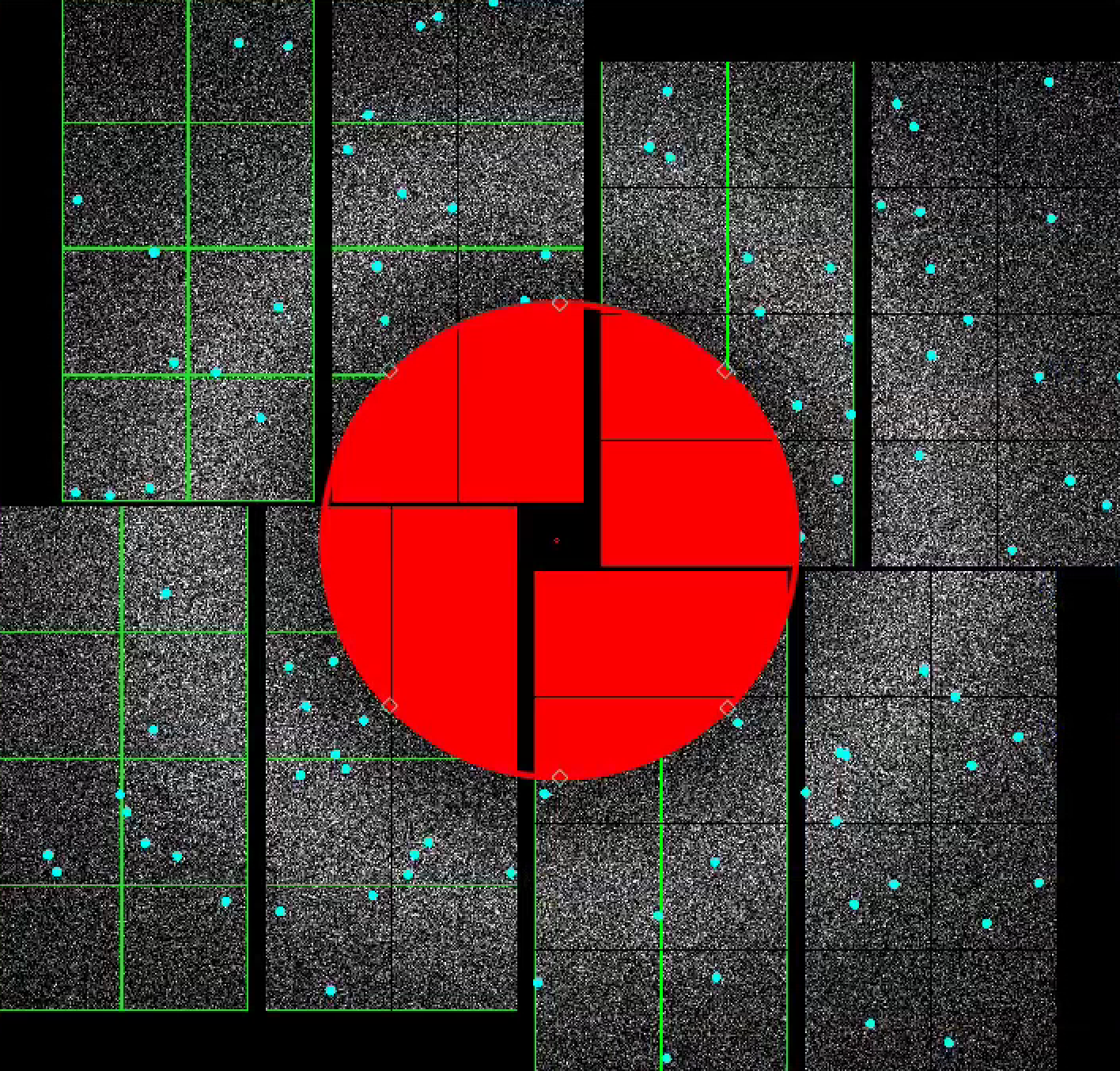
Move the red circle widget to the centre of the detector by dragging it. Resize it by dragging the diamond handle on the perimeter. Once you are happy with the area to be masked out, click "Stamp circular mask" button on the mask panel.
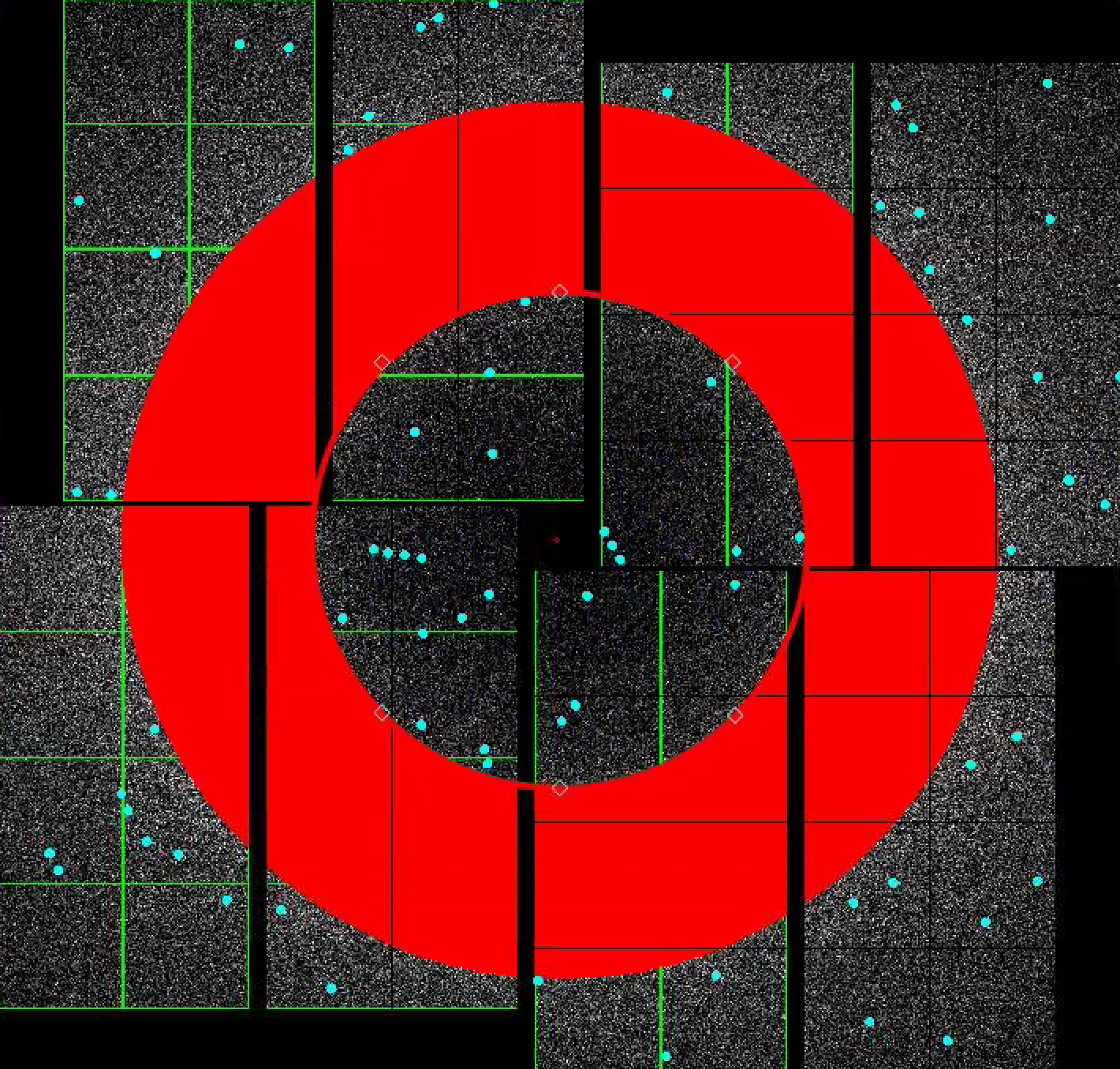
Increase the size of the red circle widget again by dragging the diamond handle on the perimeter. Click "Stamp circular mask" button on the mask panel. Because we are in the "toggle" mode, previously mask pixels inside our widget is unmasked, i.e. gets toggled. The area that does not overlap with the previous mask get masked out.
Peak finding
In this section, we will find peaks on the detector image.
Default setting in the Peak Finder panel is to "Show peaks found". You should notice peaks being highlighted in the Image panel. If you are happy with the peaks found, you are done. Otherwise, you can interactively tune peak finding parameters by expanding the "Parameters" field. Details of the peak finding algorithm is given here: Hit and Peak Finding Algorithms.
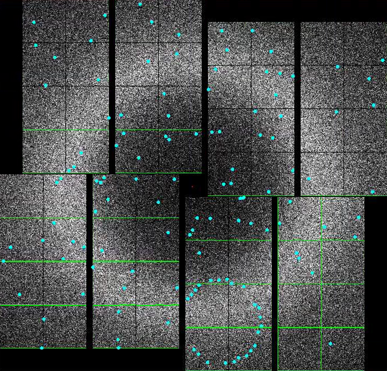
Let's optimize the peak finding parameters. Jump to event number 30 which looks like the image above. Examine the peaks found by zooming in/out with the middle mouse scroll (or a two finger slide on a Mac touchpad). Notice that the Bragg peaks are composed of 2 to 30 connected pixels. Setting the radius to 3 sets a 7x7 cyan boundary around the Bragg peaks (radius x 2+1 = 7). You can change the following values in the Peak Finder panel.
- npix_min: 2
- npix_max: 20
- radius: 3
I can see the peak finder has done a reasonable job, but missed some Bragg peaks. Hover the mouse pointer over the Bragg peaks that were not identified to study the pixel values. Let's decrease amax_thr to 140. This means every Bragg peak should have a maximum pixel that is at least 140. Let's decrease atot_thr to 300. This means a Bragg peak's pixel values will total at least 300. Let's also decrease the minimum signal-to-noise ratio (son_min) to 8.
- amax_thr: 140
- atot_thr: 300
- son_min: 8
If you have trouble finding peaks due to high background scattering, you could turn on median background subtraction. In the Experiment Parameters panel, set the Image properties to "median background corrected ADU".
Let's launch the peak finder on the cluster for a small number of events to see how this set of parameters performs. The output directory on the Peak Finder panel should already be automatically set to: /reg/d/psdm/cxi/cxic00318/scratch/<username>/psocake
Since we are analyzing run 124, /r0124 directory will be generated under the output directory.
The default setting will analyze run 124 on psanaq with 24 CPUs. Number of events to process set to -1 analyzes all the events.
For this demo, let's analyze only 50 events with 12 CPUs.
- Run(s): 124
- Queue: psanaq
- CPUs: 12
- Number of events to process: 50
Click "Launch peak finder”. To check your job progress in the queue, type the following in the terminal with your own username:
$ squeue -u <username>
For more information on which queue you are allowed to use, see Batch Nodes And Queues#BatchNodes
A logfile of the peak finding is also saved under the same directory, <jobID>.log.
If the status stays in PD or SUSP mode for awhile, then you may want to kill the jobs. To kill a batch job, type "scancel <jobID>".
You can check the status of your peak finding job here: /reg/d/psdm/cxi/cxic00318/scratch/<username>/psocake/r0124/status_peaks.txt
$ cat /reg/d/psdm/cxi/cxic00318/scratch/<username>/psocake/r0124/status_peaks.txt
{"numHits": 19, "hitRate(%)": 38.0, "fracDone(%)": 100.0}
We found 19 hits from 50 events. The hit rate is 38%. Fraction of events processed is 100%.
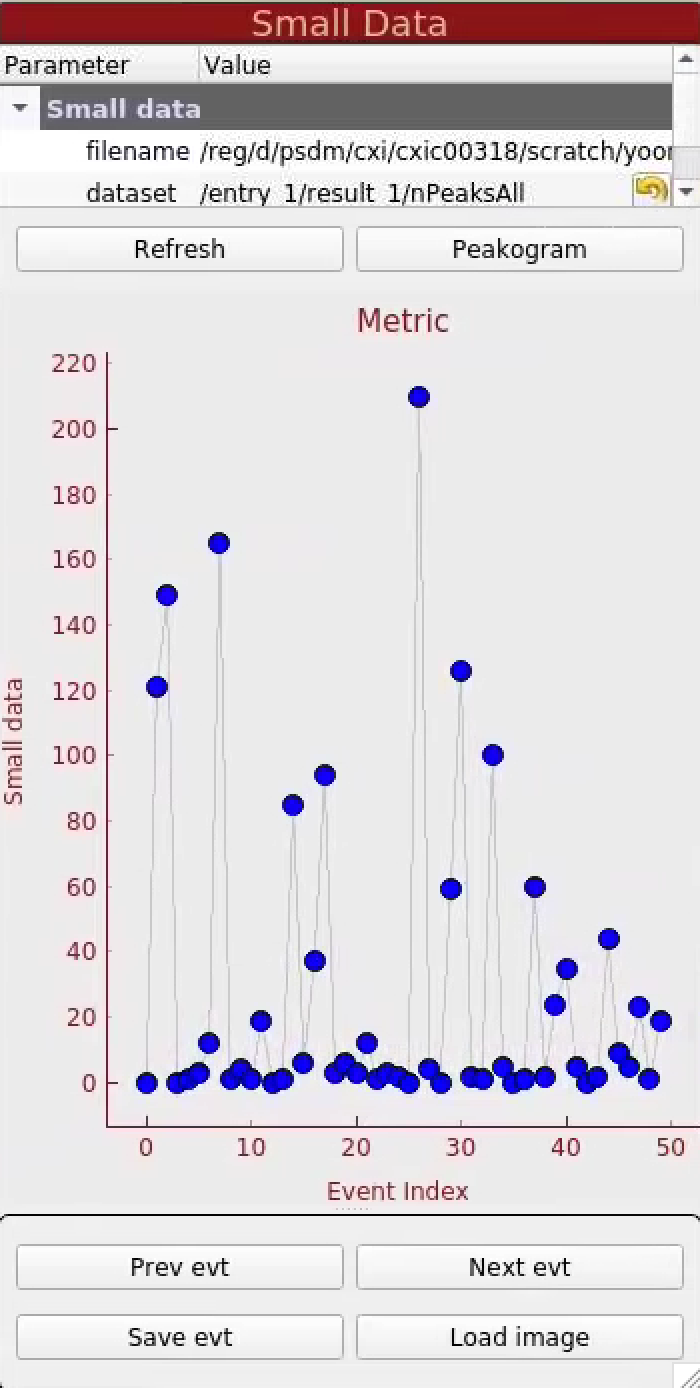
Also, click "Refresh" in Small Data panel to see the progress. You should see a red plot showing event number vs number of peaks found. When peak finding finishes, the plot will turn blue.
Note: You can launch peak finding jobs on multiple runs when you are ready to analyze the entire experiment. For example, Run(s) 1,10:13 will launch peak finding on runs 1, 10, 11, and 13.
The CXIDB file is generated in the output directory in the following format: <experiment name>_<4-digit run number>.cxi (i.e., /reg/d/psdm/cxi/cxic00318/scratch/<username>/psocake/r0124/cxic00318_0124.cxi)
Two virtual powder patterns will also be generated in the run directory:
1) cxic00318_0124_maxHits.npy: Maximum pixel values for hits found
2) cxic00318_0124_maxMisses.npy: Maximum pixel values for misses
If the hit finding parameters are good, cxic00318_0124_maxMisses.npy should not contain many Bragg spots. You can look at these images by using the "Load image" button in the Image Control panel.
Jumping to interesting images based on the number of peaks
Once you have submitted the peak finder job, let's plot the number of peaks found for each event by clicking the "Refresh" button. The refresh button will sometimes not work if your .cxi file is busy writing.
In the small data panel, you should see the CXIDB filename:
- filename: /reg/d/psdm/cxi/cxic00318/scratch/<username>/psocake/r0124/cxic00318_0124.cxi
- dataset: /entry_1/result_1/nPeaksAll
"/entry_1/result_1/nPeaksAll" is an array containing number of peaks found for each event.
This should load a plot of all the peaks found so far per event. Click "Refresh" to update the plot even if your batch job is still running.
You can click on the red marker in the plot to jump to the corresponding events.
Indexing crystals
First things first, crystal indexing requires an accurate detector geometry. Get in touch with the beamline POC if the geometry is inaccurate.
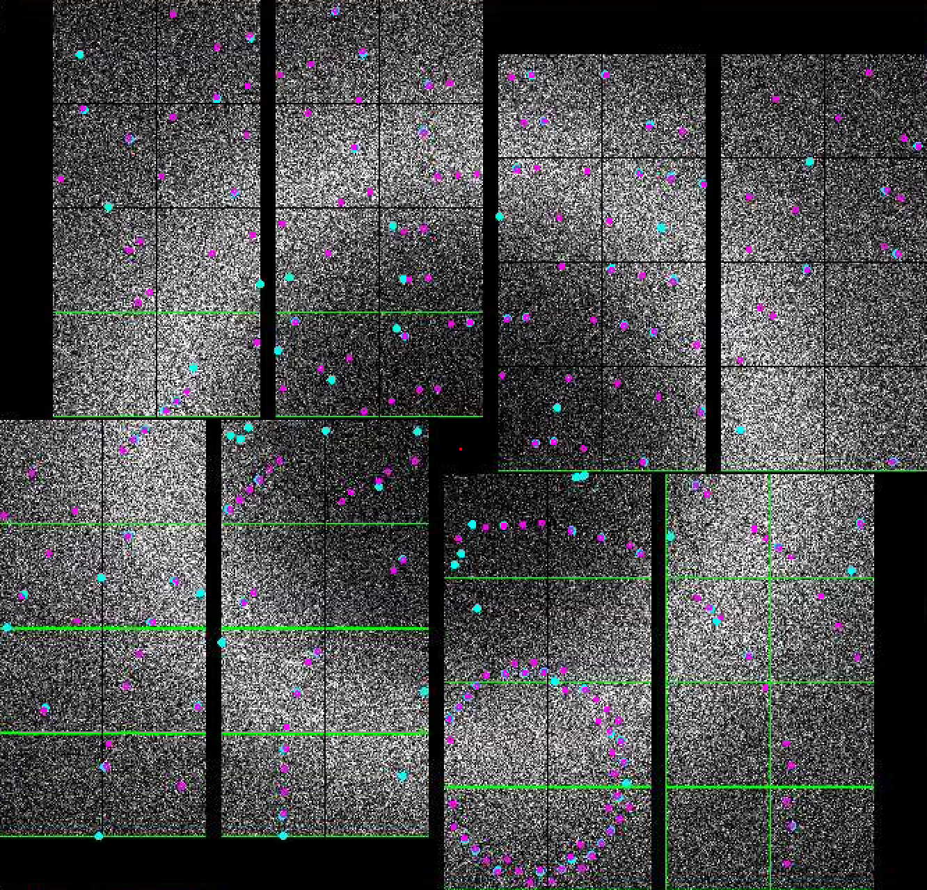
- In the indexing panel, tick "Indexing on". If indexing succeeds, the predicted peaks will be marked with magenta circles. These triple rings represent the integration radii. A large central magenta triangle means wait. If indexing fails, you will see a large central magenta X.
- If you see magenta circles and magenta unitcell appear, congratulations! You have indexed your first pattern using psocake.
- Try incrementing this distance in 1mm step till the unit cell parameters are as close as possible to lys.cell. The optimum detector distance is around 145mm.
Every time the "Detector distance" value is changed by the user, psocake converts the psana geometry (in /reg/d/psdm/cxi/cxic00318/calib/Jungfrau\:\:CalibV1/CxiDs1.0\:Jungfrau.0/geometry/123-end.data) to a CrystFEL geom file (in /reg/d/psdm/cxi/cxic00318/scratch/<username>/psocake/<runNumber>/.temp.geom).
Indexing panel uses CrystFEL to index the diffraction patterns, so the input parameters in the indexing panel should be familiar to you if you've used indexamajig before.
CrystFEL geometry: This geometry file is automatically converted from our psana geometry to CrystFEL geometry for you. Feel free to look inside .temp.geom. If you have a CrystFEL geometry file that you know is good, you can simply type it in. Psocake will never modify this file even if you change the "detector distance" in the diffraction geometry panel. (Just don't name your geometry .temp.geom, it will get overridden). You can also deploy the CrystFEL geometry as a psana geometry by clicking "Deploy CrystFEL geometry" in the indexing panel.
Integration radii: These 3 numbers define the radius of two concentric rings about each Bragg spot. Inner ring is used to integrate the Bragg spot and the outer ring is used to estimate the background. Try adjusting these numbers and see what is being integrated on screen. It should be large enough to fit a Bragg spot inside the inner ring.
PDB: If you have a CrystFEL unitcell, you can constrain the indexing algorithms to look for this unit cell.
Indexing method: Default is mosflm. You can add other indexing methods (e.g. mosflm, xds, xgandalf).
Tolerance: These 4 numbers define how much wriggle room you want for indexing. 5, 5, 5 are the tolerance level for unitcell axes a, b, c. 1.5 is the tolerance level for the angles alpha, beta, gamma.
Extra CrystFEL parameters: You can enter extra parameters for indexamajig in this field. It will be appended at the end of the command line, e.g. --profile will turn on the processing timing information.
Let's try to index another diffraction pattern at event 30.
- In the experiment parameters panel, set Event Number to 30.
- You should see the magenta triangle appear again. Wait a few seconds and hopefully you will have indexed another pattern.
Hopefully, you have indexed this diffraction pattern. Let's load a CrystFEL unitcell file to help the indexer along. Save the following text to /reg/d/psdm/cxi/cxic00318/scratch/psocake/lys.cell
CrystFEL unit cell file version 1.0
lattice_type = tetragonal
centering = P
unique_axis = c
a = 77.05 A
b = 77.05 A
c = 37.21 A
al = 90 deg
be = 90 deg
ga = 90 deg
In the Indexing panel, set the PDB field to: /reg/d/psdm/cxi/cxic00318/scratch/psocake/lys.cell
You should notice that the reindexed result will match the known unit cell parameters more closely.
Once you are happy with the detector geometry and indexing parameters, let's index the hits found in Run 124.
Make sure the peak finding has completely finished, then click "Launch indexing”.
- Run(s): 124
- Queue: psanaq
- CPUs: 24
- Keep CXI images: On
Indexing will take some time to complete. If successful, you should see a stream file in: /reg/d/psdm/cxi/cxic00318/scratch/<username>/psocake/r0124/cxic00318_0124.stream
You can check the status of your indexing job here: /reg/d/psdm/cxi/cxic00318/scratch/<username>/psocake/r0124/status_index.txt
Psocake saves the detector images of only the hits in the .cxi file. It is likely that you may want to reindex these files to optimize the indexing rate. If you anticipate that you have finalized the indexing parameters, set 'Keep CXI images' to Off. It will delete the detector images in your .cxi file which will free up your precious disk space for doing other things.
As with peak finding, you can launch indexing jobs on multiple runs by specifying runs in the Run(s) field.
Save publication images
You can save publication quality images by clicking "Save evt" button near the lower bottom right of the GUI.
Image: psocake_cxic00318_124_jungfrau4M_30_1597321015_275824216_83040_img.png
Peaks found: psocake_cxic00318_124_jungfrau4M_30_1597321015_275824216_83040_pks.png
Indexed peaks: psocake_cxic00318_124_jungfrau4M_30_1597321015_275824216_83040_idx.png
Indexing pump-probe experiments
In a pump probe experiment, it is sometimes desirable to index only certain events, e.g index only the crystals where the optical pump laser was on. This information is recorded in the EVR which psocake saves in the .cxi file (dataset name: "/LCLS/detector_1/evr1").
So if you want to index only the hits with laser on (say EVR1: 182), then type the following in the "Index condition" field:
182 in #evr1#
Psocake will also accept combinations using AND/OR:
182 in #evr1# and 173 in #evr1#
You can attach a tag to the stream filename by using the "Tag" field in the Indexing panel, e.g. evr182 would produce a new stream file cxitut13_0010_evr182.stream.
Detector centering
Let's check whether your detector is well centered with respect to your beam. You want the centre to be as accurate as possible (at least to a pixel accuracy) for optimal indexing rates.
Load the powder rings generated by clicking the "Load image" button in the Image Control panel. Open "cxic00318_0124_maxHits.npy". Adjust the intensity as necessary.
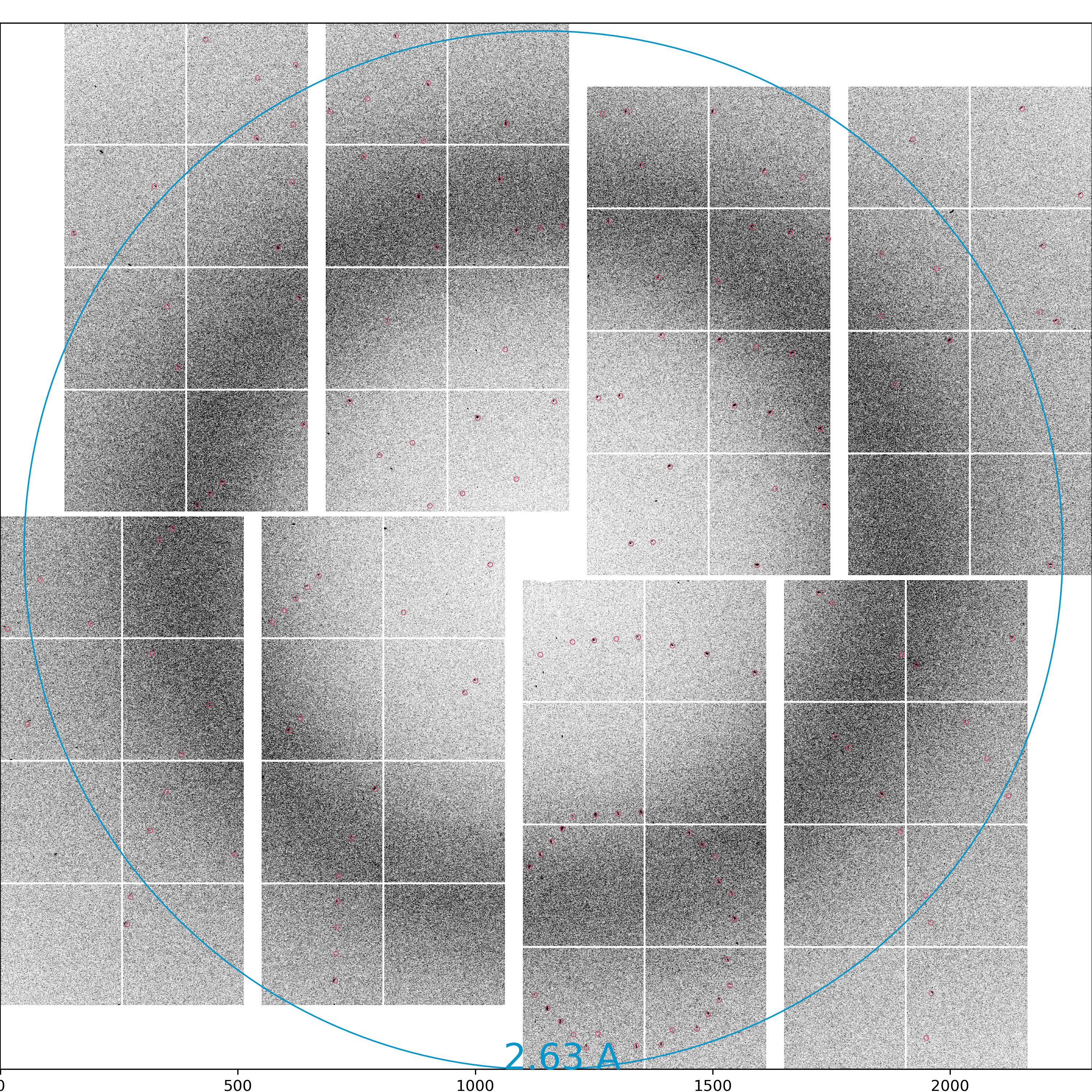
Draw resolution rings by ticking "Resolution rings" in the Diffraction Geometry panel. You can change the ring resolution by typing number in "Resolution (pixels)". Type 165 and see whether your powder rings overlap with the resolution rings. If they do, then the detector is centered. If not, then you can click on the "Deploy automatically centred geometry" to recenter your detector. If you are unhappy with the results, you can use "Deploy manually centred geometry" which will shift the detector centre to the centre of the green ROI circle.
Since we are at run124, the newly deployed geometry file is named 124-end.data. If there already exists a geometry file with the same name, it will be backed up as 124-end.data-<timeModified>
Detector geometry optimization
Past geometry files can be found here: Geometry history
It is often the case at the beginning of a beamtime that the detector distance to the interaction point (coffset) is not precisely known (we are talking about sub-millimetre precision), and we can use the Diffraction Geometry panel to find the optimal distance.
Post-processing
Once you are satisfied with indexing all your runs, please remember to backup your .cxi files in the /res directory of your experiment. The scratch folder will get wiped after few months (Data Retention Policy).
The stream file is small enough to transfer back to your institute for post-processing (CrystFEL tutorial) and phase retrieval (PHENIX).
For phase retrieval, you can use Phenix and CCP4 by sourcing the following lines:
# Phenix (version number may change)
source /reg/common/package/phenix/phenix-1.10.1-2155/phenix_env.sh
# CCP4 (version number may change)
source /reg/common/package/ccp4/ccp4-7.0/bin/ccp4.setup-sh
# XDS is available here
/reg/common/package/XDS-INTEL64_Linux_x86_64/
For viewing the electron density, use coot contained inside phenix.
Beam Parameters for Publications
You can use psana to retrieve EPICS variables that are used in SFX publications, such as the pulse energy and the number of photons per pulse.
Common EPICS variables for SFX
ebeam = ebeamDet.get(evt)
pulseEnergy = ebeam.ebeamL3Energy()  # MeV

es = psana.DataSource.env().epicsStore()
calculatedNumberOfPhotons = get_es_value(es, 'SIOC:SYS0:ML00:AO580', NoneCheck=False, exceptReturn=0) * 1e12  # photons
Bug/Comments:
Please send bug reports/comments:
Tiny url for this tutorial: http://tinyurl.com/zj4m23n
Overview
Content Tools