This note is about n-d array processing algorithms implemented in ImgAlgos.PyAlgos. Algorithms can be called from python but low level implementation is done on C++ with boost/python wrapper. All examples are shown for python level interface.
Content
Common features of algorithms
n-d arrays
LCLS detector data come from DAQ as n-d arrays (ndarray in C++ or numpy.array in Python). In simple case camera data is an image presented by the 2-d array. For composite detectors like CSPAD, CSPAD2X2, EPIX, PNCCD, etc. data comes from a set of sensors as 3-d or 4-d arrays. If relative sensors' positions are known, then sensors can be composed in 2-d image. But this image contains significant portion of "fake" empty pixels, that may be up to ~20-25% in case of CSPAD. Most efficient data processing algorithms should be able to work with n-d arrays.
Windows
In some experiments not all sensors contain useful data. It might be more efficient to select Region of Interest (ROI) on sensors, where data need to be processed. To support this feature a tuple (or list) of windows is passed as a constructor parameter. Each window is presented by the tuple of 5 parameters (segnum, rowmin, rowmax, colmin, colmax), where segnum is a sensor index in the n-d array, other parameters constrain window 2-d matrix rows and columns. Several windows can be defined for the same sensor using the same segnum. For 2-d arrays segnumparameter is not used, but still needs to be presented in the window tuple by any integer number. To increase algorithm efficiency only pixels in windows are processed. If windows=None, all sensors will be processed.
The array of windows can be converted in 3-d or 2-d array of mask using method pyimgalgos.GlobalUtils.mask_from_windows.
Mask
Alternatively ROI can be defined by the mask of good/bad (1/0) pixels. For 2-d image mask can easily be defined in user's code. In case of ≥3-d arrays the Mask Editor helps to produce ROI mask. Entire procedure includes
- conversion of n-d array to 2-d image using geometry,
- production of ROI 2-d mask with Mask Editor,
- conversion of the 2-d mask to the mask n-d array using geometry.
All steps of this procedure can be completed in Calibration Management Tool under the tab ROI.
In addition mask accounts for bad pixels which should be discarded in processing. Total mask may be a product of ROI and other masks representing good/bad pixels.
Make object and set parameters
Any algorithm object can be created as shown below.
import numpy as np
from ImgAlgos.PyAlgos import PyAlgos

# create object:
alg = PyAlgos(windows=winds, mask=mask, pbits=0)
Define ROI using windows and/or mask
Region Of Interest (ROI)is defined by the set of rectangular windows on segments and mask, as shown in example below.
# List of windows
winds = None # entire size of all segments will be used for peak finding
winds = (( 0, 0, 185, 0, 388),
         ( 1, 20,160, 30,300),
         ( 7, 0, 185, 0, 388))

# Mask
mask = None                   # (default) all pixels in windows will be used for peak finding
mask = det.mask()             # see class Detector.PyDetector
mask = np.loadtxt(fname_mask) #
mask.shape = <should be the same as shape of data n-d array>
Hit finders
Hit finders return simple values for decision on event selection. Two algorithms are implemented in ImgAlgos.PyAlgos. They count number of pixels and intensity above threshold in the Region Of Interest (ROI) defined by windows and mask parameters in object constructor.
Both hit-finders receive input n-d drray data and threshold thr parameters and return a single value in accordance with method name.
Number of pixels above threshold
number_of_pix_above_thr
npix = alg.number_of_pix_above_thr(data, thr=10)
Total intensity above threshold
intensity_of_pix_above_thr
intensity = alg.intensity_of_pix_above_thr(data, thr=12)
Peak finders
Peak finder works on calibrated, background subtracted n-d array of data in the region of interest specified by the list of windows and using only good pixels from mask n-d array. All algorithms implemented here have three major stages
- find a list of seed peak candidates
- process peak candidates and evaluate their parameters
- apply selection criteria to the peak candidates and return the list of peaks with their parameters
The list of peaks contains 17 (float for uniformity) parameters per peak:
- seg - segment index beginning from 0, example for CSPAD this index should be in the range (0,32)
- row - index of row beginning from 0
- col - index of column beginning from 0
- npix - number of pixels accounted in the peak
- amp_max - pixel with maximal intensity
- amp_total - total intensity of all pixels accounted in the peak
- row_cgrav - row coordinate of the peak evaluated as a "center of gravity" over pixels accounted in the peak using their intensities as weights
- col_cgrav - column coordinate of the peak evaluated as a "center of gravity" over pixels accounted in the peak using their intensities as weights
- raw_sigma - row sigma evaluated in the "center of gravity" algorithm
- col_sigma - column sigma evaluated in the "center of gravity" algorithm
- row_min - minimal row of the pixel group accounted in the peak
- row_max - maximal row of the pixel group accounted in the peak
- col_min - minimal column of the pixel group accounted in the peak
- col_max - maximal column of the pixel group accounted in the peak
- bkgd - background level estimated as explained in section below
- noise - r.m.s. of the background estimated as explained in section below
- son - signal over noise ratio estimated as explained in section below
There is a couple of classes helping to save/retrieve peak parameter records in/from the text file:
Peak selection parameters
Internal peak selection is done at the end of each peak finder, but all peak selection parameters need to be defined right after algorithm object is created. These peak selection parameters are set for all peak-finders:
# create object:
alg = PyAlgos(windows=winds, mask=mask)

# set peak-selector parameters:
alg.set_peak_selection_pars(npix_min=5, npix_max=5000, amax_thr=0, atot_thr=0, son_min=10)
- npix_min: minimum number of pixels that pass the "low threshold" cut
- npix_max: maximum number of pixels that pass the "low threshold" cut
- amax_thr: pixel value must be greater than this high threshold to start a peak
- atot_thr: to be considered a peak the sum of all pixels in a peak must be greater than this value
- son_min: required signal-over-noise (where noise region is typically evaluated with radius/dr parameters). set this to zero to disable the signal-over-noise cut.
All peak finders have a few algorithm-dependent parameters
Two threshold "Droplet finder"
two-threshold peak-finding algorithm in restricted region around pixel with maximal intensity. Two threshold allows to speed-up this algorithms. It is assumed that only pixels with intensity above thr_high are pretending to be peak candidate centers. Candidates are considered as a peak if their intensity is maximal in the (square) region of radius around them. Low threshold in the same region is used to account for contributing to peak pixels.
peak_finder_v1
peaks = alg.peak_finder_v1(nda, thr_low=10, thr_high=150, radius=5, dr=0.05)
Parameter radius in this algorithm is used for two purpose:
- defines (square) region to search for local maximum with intensity above
thr_highand contributing pixels with intensity abovethr_lo, - is used as a
r0parameter to evaluate background and noise rms as explained in section below.
peak_finder_v4
peaks = alg.peak_finder_v4(nda, thr_low=10, thr_high=150, rank=4, r0=5, dr=0.05)
The same algorithm as peak_finder_v1 , but parameter radius is split for two (unsigned) rank and (float)r0 with the same meaning as in peak_finder_v3 .
Flood filling algorithm
define peaks for regions of connected pixels above threshold
peak_finder_v2
peaks = alg.peak_finder_v2(nda, thr=10, r0=5, dr=0.05)
Two neighbor pixels are assumed connected if have common side. Pixels with intensity above threshold thr are considered only.
Local maximums search algorithm
define peaks in local maximums of specified rank (radius), for example rank=2 means 5x5 pixel region around central pixel.
peak_finder_v3
peaks = alg.peak_finder_v3(nda, rank=2, r0=5, dr=0.05)
- makes a map of pixels with local maximums of requested rank for data ndarray and mask, pixel code in the map may have bits 0/1/2/4 standing for not-a-maximum / maximum-in-row / maximum-in-column / maximum-in-rectangular-region of radius=rank.
- for each pixel with local maximal intensity in the region defined by the rank radius counts a number of pixels with intensity above zero, total positive intensity, center of gravity coordinates and rms,
- using parameters
r0(ex.=5.0), dr(ex.=0.05)evaluates background level, rms of noise, and S/N for the pixel with maximal intensity. - makes list of peaks which pass selector with parameters set in
set_peak_selection_pars, for example
alg.set_peak_selection_pars(npix_min=5, npix_max=500, amax_thr=0, atot_thr=1000, son_min=6)
Demonstration for local maximum map
Test for 100x100 image with random normal distribution of intensities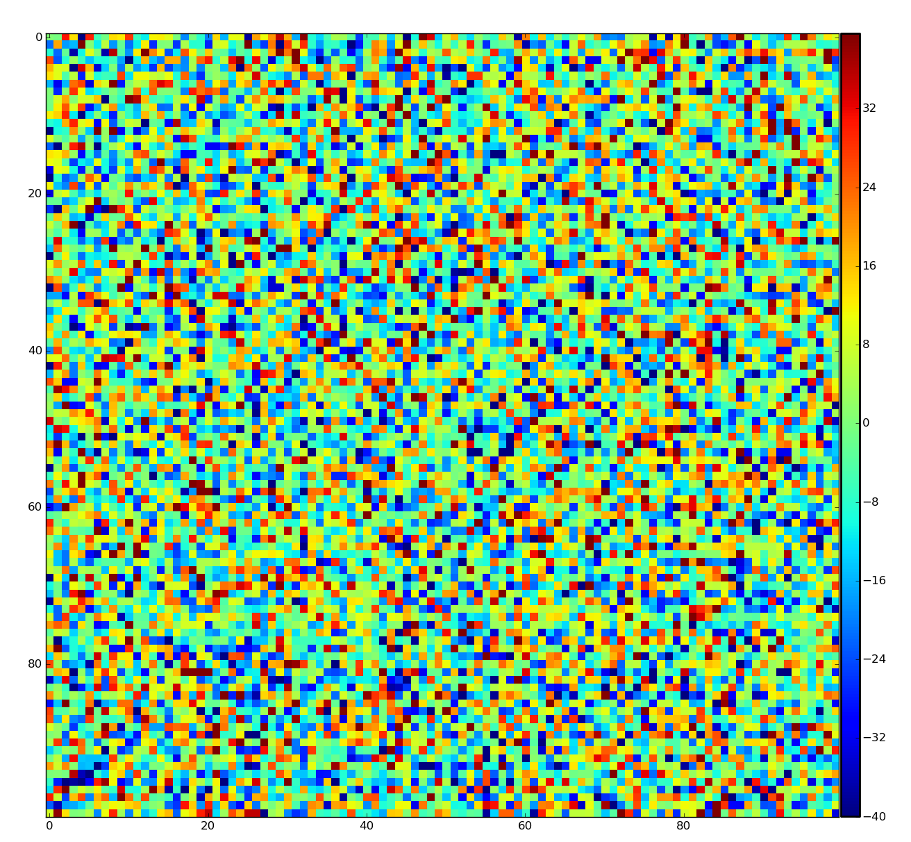
Example of the map of local maximums found for rank from 1 to 5:
![]()
![]()
![]()
![]()
![]()
color coding of pixels:
- blue=0 - not a local maximum
- green=1 - local maximum in row
- yellow=1+2 - local maximum in row and column
- red=1+2+4 - local maximum in rectangular region of radius=rank.
Table for rank, associated 2-d region size, fraction of pixels recognized as local maximums for rank, and time consumption for this algorithm.
| rank | 2-d region | fraction | time, ms |
|---|---|---|---|
| 1 | 3x3 | 0.1062 | 5.4 |
| 2 | 5x5 | 0.0372 | 5.2 |
| 3 | 7x7 | 0.0179 | 5.1 |
| 4 | 9x9 | 0.0104 | 5.2 |
| 5 | 11x11 | 0.0066 | 5.2 |
Evaluation of the background level, rms, and S/N ratio
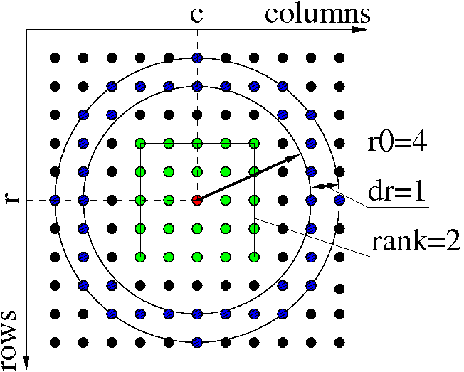
When peak is found, its parameters can be precised for background level, noise rms, and signal over background ratio (S/N) can be estimated. All these values can be evaluated using pixels surrounding the peak on some distance. For all peak-finders we use the same algorithm. Surrounding pixels are defined by the ring with internal radial parameter r0 and ring width dr (both in pixels). The number of surrounding pixels depends on r0 and dr parameters as shown in matrices below. We use notation
- + central pixel with maximal intensity,
- 1 pixels counted in calculation of averaged background level and noise rms,
- 0 pixels not counted.
Matrices of pixels for r0=3 and 4 and different dr values
Matrices of pixels for r0=5 and 6 and different dr values
Matrix of pixels for r0=7
Test of peak finders
Photon counting
Photon conversion in pixel detectors is complicated by the split photons between neighboring pixels. In some cases, energy deposited by a photon is split between two or (sometimes) more pixels. The photon counting algorithm described here is designed to account for this effect and return an unassembled array with correct number of photons per pixel. Pythonic API for this algorithm is as follows:
# Import
import psana

# Initialize a detector object
det = psana.Detector('myAreaDetectorName')
# Merges photons split among pixels and returns n-d array with integer number of photons per pixel.
nphotons_nda = det.photons(evt, nda_calib=None, mask=None, adu_per_photon=None)
The det.photons() function divides the pixel intensities (ADUs) by adu_per_photon, resulting in a fractional number of photons for each pixel. This function is a wrapper around photons() method in PyAlgos:
# Import
from ImgAlgos.PyAlgos import photons

# Merges photons split among pixels and returns n-d array with integer number of photons per pixel.
nphotons_nda = photons(fphotons, adu_per_photon=30)
Method photons receives (float) n-d numpy array fphotons representing image intensity in terms of (float) fractional number of photons and an associated mask of bad pixels. Both arrays should have the same shape. Two lowest dimensions represent pixel rows and columns in 2-d pixel matrix arrays. Algorithm works with good pixels defined by the mask array (1/0 = good/bad pixel). Array fphotons is represented with two arrays; An array containing whole number of photons (integer) and the leftover fractional number of photon array (float) of the same shape. Assuming the photons are only split between two adjacent pixels, we round up the adjacent pixels if they sum up to be above 0.9 photons. The algorithm is best explained using an example:
Let's say we measured the following ADUs on our detector. "adu_per_photon" is user-defined, but for this example let's set it to 1:
ADUs (adu_per_photon=1):
0.0 3.5 0.1 0.2
0.2 0.4 0.0 1.2
0.1 4.7 3.4 0.0
0.5 0.4 0.4 0.1
We expect the converted photon counts to be:
Photons:
0 4 0 0
0 0 0 1
0 5 3 0
1 0 0 0
To see how we get from ADUs to Photons, we split the ADUs into whole photons and fractional photons.
ADUs               =  Whole photons   +    Fractional photons
0.0 3.5 0.1 0.2          0 3 0 0              0.0 0.5 0.1 0.2
0.2 0.4 0.0 1.2    =     0 0 0 1      +       0.2 0.4 0.0 0.2
0.1 4.7 3.4 0.0          0 4 3 0              0.1 0.7 0.4 0.0
0.5 0.4 0.4 0.1          0 0 0 0              0.5 0.4 0.4 0.1
Assuming the photons are only split by two adjacent pixels, we search for a pixel that has at least 0.5 photons with an adjacent pixel that sum up to above 0.9 photons. In cases where a pixel has multiple adjacent pixels which sum up to above 0.9 photons, we take the largest adjacent pixel. If such an adjacent pair of pixels is found, then the adjacent pixel values are merged into one pixel. It is merged into the pixel with the larger value. (See "After merging adjacent pixels" example below).
The merged adjacent pixels are then rounded to whole photons. (See "Rounded whole photons" example below).
Fractional photons
0.0 0.5 0.1 0.2
0.2 0.4 0.0 0.2
0.1 0.7 0.4 0.0
0.5 0.4 0.4 0.1

After merging adjacent pixels:
0.0 0.9 0.1 0.2
0.2 0.0 0.0 0.2
0.1 1.1 0.0 0.0
0.9 0.0 0.4 0.1

Rounded whole photons:
0 1 0 0
0 0 0 0
0 1 0 0
1 0 0 0
Photons is then the sum of "Whole photons" and "Rounded whole photons":
Photons = Whole photons + Rounded whole photons:
0 4 0 0      0 3 0 0       0 1 0 0
0 0 0 1  =   0 0 0 1   +   0 0 0 0
0 5 3 0      0 4 3 0       0 1 0 0
1 0 0 0      0 0 0 0       1 0 0 0
References
- ImgAlgos.PyAlgos - code documentation
- psalgos - new peak-finder and other algorithms code documentation
- Peak Finding - short announcement about peak finders
- Hit and Peak Finders - examples in Chris' tutorial
- GUI for tuning peak finding - Chun's page in development
- Auto-generated documentation - references to code-based documentation for a few other useful packages
pyimgalgos.PeakStore - class helping to save peak parameter records in the text file
pyimgalgos.TDFileContainer - class helping to retrieve peak parameter records from the text file
Test of Peak Finders - example of exploitation of peak finders
- Test of Peak Finders - V2 - example of exploitation of peak finders after revision 1 (uniformization)
- photons - sphinx doc
- Peak Finding Module - (depricated) psana module, it demonstaration examples and results
- Psana Module Catalog - (depricated) peak finding psana modules
- Psana Module Examples - (depricated) peak finding examples in psana modules
Overview
Content Tools