This note describes imaging detectors' hierarchical geometry model which is implemented in LCLS offline software since release ana-0.13.1.

Content

Introduction

Analysis of LCLS data from imaging experiments requires precise coordinate definition of the photon detection spot. In pixel array detectors photon energy usually deposited in a single pixel and hence pixel location precision should be comparable or better than its size, about 100μm. Apparently, calibration of the detector and entire experimental setup geometry with such a precision is a challenging task for many reasons;

position of the detector sensors relative to interaction point (IP) of the photon beam with target is not well known,
in some cases detector is a composition of other sub-detectors arranged together and consisting of other sub-detectors and so on for a few layers in depth,
sub-detectors of each layer may have stable positions or be moved by stepping motor relative to each other,
final level sub-detector is represented by precisely engineered sensor(s) of particular type(s) which geometry needs to be tabulated.

To take into account this structure we may consider a variable length series of hierarchical objects like sensor -> sub-detector -> detector -> setup, where lower-level child object(s) is(are) embedded in its higher-level parent object. Nodes/objects of this hierarchical model form the tree which is convenient for navigation and recursion algorithms. Each child object location and orientation can be described in the parent frame. Tree-like structure can be kept in form of table saved in and retrieved from file. The last feature is practically useful for calibration purpose. All constants for detector/experiment geometry description can be saved in a single file. Relevant parts of the hierarchical table can be calibrated and updated whenever new geometry information is available, for example from optical measurement or dedicated runs with images of bright diffraction rings or Bragg peaks.

This note contains description of the implemented hierarchical geometry model, coordinate transformation algorithms, tabulation of the hierarchical objects and calibration file format, description of software interface in C++ and Python, details of calibration, etc.

Coordinate frames

In this section we list tentative objects and associated coordinate frames which may be involved in typical LCLS experimental setup and explain how they can be inscribed in the hierarchical model.

Experimental setup

On the very top level of hierarchical structure there should be a global coordinate frame associated with entire experimental setup. All other setup components are defined relative to the global coordinate frame. In diffraction experiments origin of the coordinate frame is usually associated with IP. Choice of axes directions depends on experimental preferences. In some of LCLS experiments Cartesian coordinate system of the setup is defined by the three mutually orthogonal right-hand-indexed axes with origin in the IP:

X axis pointing from IP to the north,
Y axis pointing from IP to the top, and
Z axis pointing from IP along the photon beam propagation direction,

as shown in the plot:

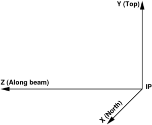FIG. 1: Tentative coordinate frame of experimental setup.

In this frame photon-hit pixel coordinates (x, y, z) can be easily transformed to the photon diffraction angle θ,

Sensor

On the very bottom level of hierarchy structure there should be self-sufficient components of the detector - sensors a.k.a. tiles, segments, pixel arrays/matrix etc. We assume that

tiles may be of different types even in a single detector,
all tiles of the same type have identical geometry,
by design each tile has well defined geometry of pixels which does not need in calibration,
pixel center (x, y, z) coordinates in each tile can be defined as a look-up table for all pixels,
each tile is represented in data as a minimal solid block of memory,
“natural” matrix-style pixel numeration is preferable for simplicity of the tile description but is not necessarily required.

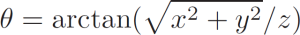
For example, CSPAD 2x1 tile pixel geometry is schematically shown below

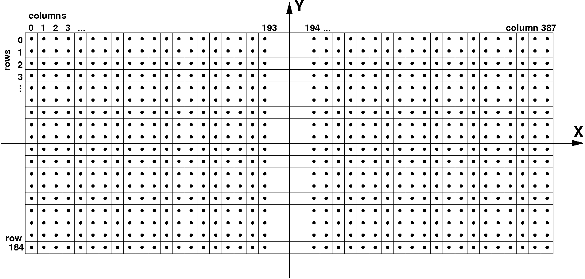FIG. 2: Coordinate frame of CSPAD 2x1 sensor.

The CSPAD 2x1 tile has

185 rows and 388 columns of pixels,
regular pixel size is 109.92 × 109.92 μm²,
pixel size in two middle columns 193 and 194 is 274.80 × 109.92 μm².

The pixel index and coordinates in the tile memory block of size 185×388 can be evaluated as

y = k * row + y_offset

x = f(column)

where y coordinate is proportional to the row index, while x coordinate needs to be tabulated as a function of the column index due to the gap in the tile central columns braking matrix uniformity. Detector data record consists of consecutive tile-memory blocks, in accordance with numeration adopted in DAQ. For effective memory management, some of the tile-blocks may be missing due to current detector configuration. Available configuration of the detector tile-blocks should be marked in a configuratiomn bit-mask word in positional order (bit position from lower to higher is associated with the tile number in DAQ).

Child geometry object in the parent frame

Full description of a composite detector (beside top and bottom level hierarchical objects) needs in definition of intermediate objects with their arbitrary location and orientation. Any geometry object coordinate system may have a translation and rotation with respect to the parent object, which can be defined by the 3 vectors in the setup frame as shown in Figure

FIG. 3: Child object position in the parent coordinate frame.

where

P is a translation vector pointing from parent to its child frame origin,
e_x is a unit vector along the child frame x axis,
e_y is a unit vector along the child frame y axis.

Third unit vector e_z is assumed to be right-hand triplet component, 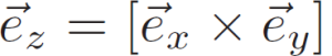. Components of these three unit vectors form the rotation matrix

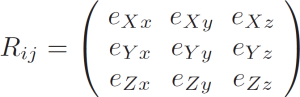
where index “j” enumerates unit vectors in the object coordinate frame, and index “i” is an object unit vector component in the parent frame (ex.: e_Yz is a Y component of the vector e_z). Within this definition 3-d pixel coordinate “c” in the object frame can be transformed to the parent coordinate frame “C” using equation

C_i=R_ij·c_j + P_i.

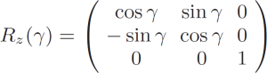
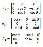
For practical reason we parametrize rotation matrix Rij in terms of Cardan’s angles R(α, β, γ). We assume that the 3-d rotation matrix R(α, β, γ) is a product of three 2-d rotations

R(α, β, γ) = Rx(α) · Ry(β) · Rz(γ),

around appropriate axes, defined as

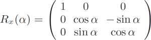
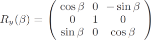
This transformation algorithm is implemented in class PSCalib.GeometryObject as discussed below.

Example of composite detector

As an example we show how composite CXI-like CSPAD detector with moving quads can be inscribed in the hierarchical geometry model and how geometry parameters can be retrieved in each level.

CSPAD 2x1 sensor (Fig. 2) is the low-level object with completely specified geometry of pixels.
A group of eight cspad 2x1 sensors forms a quad (Fig. 4). Sensors’ positions in the quad can be measured by optical microscope.
Four quads form a CSPAD detector. In CXI-like CSPAD quads can be moved by the stepping motor. For technical reason this detector can not be measured with optical microscope. Dedicated runs with bright images of test wires, diffraction rings, or Bragg peaks can be used to calibrate relative quad positions. Then, quads’ position variation by the stepping motor can be accounted for once calibrated quads.
Finally, detector position relative to IP should be accounted (Fig. 6). Detector position and orientation can be measured by the ruler in the hatch for the first approximation. The same dedicated runs with bright images can be used to evaluate precise detector coordinates. Calibration runs with a few detector positions along the beam line can be helpful for full geometry parameters reconstruction.

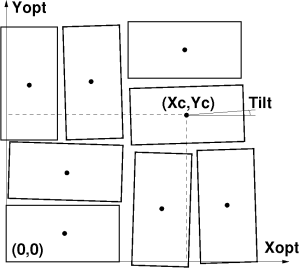FIG. 4: Example: 2x1 sensors’ positions in the CSPAD quad coordinate frame.

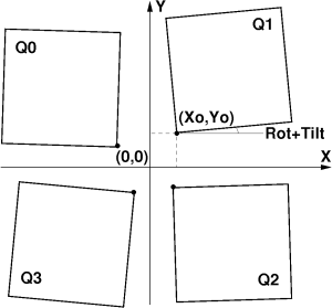FIG. 5: Example: quads’ positions in the CSPAD detector coordinate frame.

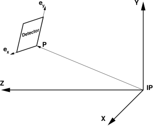FIG. 6: Example: detector position in the experiment coordinate frame with origin at IP.

Optical measuremets

Precise pixel coordinates can be retrieved in a few steps using

ideal tile design geometry (Fig. 2),
results of measurements with optical microscope,
correction of sub-detector elements using dedicated runs.

In this section we describe a procedure of optical measurements, its potential problem, and method to fix it.

Metrology file

Optical measurements with microscope give the most precise information about sensors’ positions in the parent structure. Estimated accuracy of measurements is σRMS ∼ 10μm in x-y plane, and about the same amount in z. Optical measurements provide 3-d coordinates of 4 corners for all tiles in the (sub-)detector in some arbitrary microscope plane which coincides with detector imaging array (tiles) plane within precision of installation.

Tile corner coordinates do not necessarily coincide with pixel centers or corners.
Numeration of tiles in optical measurements should not necessarily coincide with their numeration in DAQ, but it should be done in expected order with indication of tile numbers.
Optical measurements are saved in the xlsx file as a table of x, y, z coordinates for all sensor corners with records like

Tile <#>

Point <#> <X[um]> <Y[um]> <Z[um]>

Metrology files are produced by the detector group for new or repaired detectors.

Quality check

Measurements with microscope are not automated. Results are manually saved in the metrology file, which may have non-intentional typos. If the number of typos is small they can be tracked down in the quality check and fixed. Quality check of optical measurement may test for each tile:

equity of opposite sides
equity of diagonals
equity of tilt angles for all sides
tile flatness in 3-d

Report table about all deviations is generated by the python script processing the metrology file. Large deviations exceeding standard precision >3σ(RMS) indicate on problem with measurement. A few corrections are usually applied for each metrology file.

Position of tiles in the detector

Detector pixels' geometry in 3-d can be unambiguously derived from

the list of coordinates obtained in optical measurements,
tile ideal geometry, and
designed orientation of sensors in the detector.

The tile location and orientation can be defined by the table of records (see example of file: geometry/0-end.data)

Parent name	Parent index	Object name	Object index	X0[µm]	Y0[µm]	Y0[µm]	Rotation Z [°]	Rotation Y [°]	Rotation X[°]	Tilt Z[°]	Tilt Y[°]	Tilt X[°]

where

Parent name - name and version of the parent object; all translation and rotation pars are defined w.r.t. parent Cartesian frame
Parent index - index of the parent object
Object name - name and version of the object inserted in parent frame
Object index - index of the object
X0, Y0, and Z0 [µm] – object frame origin coordinates in the parent frame
Rotation X, Y, and Z [degree] – object ideal (design) rotation angle around axes Z, Y, and X of the parent frame
Tilt X, Y, and Z [degree] – tilt angles for correction of the object rotation angles around axes Z, Y, and X of the parent frame, respectively

Tile center coordinates are defined as an average over 4 corners. Tilt angles are projected angles of the tile sides on relevant planes. Each angle is evaluated as an averaged angle for 2 sides.

Origin of the detector local frame is arbitrary. For example, for CSPAD with moving quads it is convenient to define

2x1 sensors' centre coordinates in the quad coordinate system as in optical measurements,
quad origins' coordinates with respect to the point of beam crossing with the detector plane (centre of the diffraction rings), as shown on plots:

Pixel coordinates reconstruction

Pixel coordinate reconstruction in the detector frame uses

tile ideal geometry,
tile center positions,
tile N·90 rotation and tilt angles.

Each geometry object pixel coordinate x_j are transformed to the parent frame pixel coordinate X_iapplying rotations and translations as
X_i=R_ij·_xj + P_i,

or in Python code:

#file: pyimgalgos/src/GeometryObject.py

def rotation(X, Y, C, S) :
    Xrot = X*C - Y*S 
    Yrot = Y*C + X*S 
    return Xrot, Yrot

class GeometryObject :
    ...
    def transform_geo_coord_arrays(self, X, Y, Z) :
        ...
	    # define Cx, Cy, Cz, Sx, Sy, Sz - cosines and sines of rotation + tilt angles
        ...

        X1, Y1 = rotation(X,  Y,  Cz, Sz)
        Z2, X2 = rotation(Z,  X1, Cy, Sy)
        Y3, Z3 = rotation(Y1, Z2, Cx, Sx)

        Zt = Z3 + self.z0
        Yt = Y3 + self.y0
        Xt = X2 + self.x0

        return Xt, Yt, Zt

where the 3-d rotation matrix R is a product of three 2-d rotations around appropriate axes,

Pixel coordinates in the detector should be accessed by the method like

xarr, yarr, zarr = get_pixel_coords()

For example, Python interface for CSPAD

from pyimgalgos.GeometryAccess import GeometryAccess
    ...
    fname_geometry='<path>/geometry/0-end.data'
    geometry = GeometryAccess(fname_geometry)
    X,Y,Z = geometry.get_pixel_coords()

will return X,Y,Z arrays of the shape [4,8,185,388], or similar for CSPAD quad, one has to show the top object for coordinate arrays, say it is 'QUAD:V1' with index 1:

    geometry = GeometryAccess(fname_geometry)
    X,Y,Z = geometry.get_pixel_coords('QUAD:V1', 1)

return X,Y,Z arrays of the shape [8,185,388].

Software

Interface description is available in doxygen

Geometry file producer

CalibManager.OpticAlignmentCspadV1.py - for cxi-CSPAD
TBD for xpp-CSPAD, ePix, etc. whenever available

Alignment

TBD: under CalibManager.GUIGeometry.py

Hierarchical geometry model in C++

PSCalib::SegGeometry - Interface definition of the pixel geometry for basic segments/sensors
PSCalib::SegGeometryStore - static factory method for switching between different devices
PSCalib::SegGeometryCspad2x1V1 - defines 2x1 pixel geometry through the base class SegGeometry interface methods
PSCalib::GeometryObject,
PSCalib::GeometryAccess,

Hierarchical geometry model in Python

The same package and file names as in C++ but with file name extension .py:

PSCalib/src/*.py

Summary

Suggested method for imaging detector geometry description provides simple and unambiguous way of pixel coordinate parametrization. This method utilizes all available information from optical measurement and design of the detector and tiles. All geometry parameters are extracted without fitting technique and presented by natural intuitive way.

References

Euler angles, Tait–Bryan angles, nautical angles, Cardan angles etc.
Imaging Detector Geometry Implementation Notes
Example of the file for calibration type geometry/0-end.data

Reference to doxygen documentation of classes

Imaging Detector Geometry Description