This note describes imaging detectors' hierarchical geometry model implemented in LCLS offline software releases since ana-0.13.1.
Content
Introduction
Note that public detector geometry data can be found here.
Nearly all imaging experiments conducted at LCLS require a precise description of the experimental geometry, especially how one or more area detectors are arranged with respect to the x-ray beam and interaction site. In pixel array detectors photon energy is usually deposited in a single pixel and hence a description of the experimental geometry should aim to provide the pixel location to a precision comparable with or better than its size, for the CSPAD about 100μm.
Determination of the experimental geometry to such a precision is a challenging task for many reasons:
- position of the detector sensors relative to interaction point (IP) of the photon beam with target is not well known,
- in some cases detector is a composition of other sub-detectors arranged together and consisting of other sub-detectors and so on,
- sub-detectors of each layer may have stable positions or be moved by stepping motor relative to each other,
- final level sub-detector is represented by precisely engineered sensor(s) of particular type(s) which geometry needs to be tabulated.
To take into account this structure we may consider a variable length series of hierarchical objects like sensor -> sub-detector -> detector -> setup, where lower-level child object(s) is(are) embedded in its higher-level parent object. Nodes/objects of this hierarchical model form the tree which is convenient for navigation and recursion algorithms. Each child object location and orientation can be described in the parent frame. Tree-like structure can be kept in form of table saved in and retrieved from file. The last feature is practically useful for calibration purpose. All constants for detector/experiment geometry description can be saved in a single file. Relevant parts of the hierarchical table can be calibrated and updated whenever new geometry information is available, for example from optical measurement or dedicated runs with images of bright diffraction rings or Bragg peaks.
This note contains description of the implemented hierarchical geometry model, coordinate transformation algorithms, tabulation of the hierarchical objects and calibration file format, description of software interface in C++ and Python, details of calibration, etc.
Coordinate frames
In this section we list tentative objects and associated coordinate frames which may be involved in typical LCLS experimental setup and explain how they can be inscribed in the hierarchical model.
Experimental setup
On the very top level of hierarchical structure there should be a global coordinate frame associated with entire experimental setup. All other setup components are defined relative to the global coordinate frame. In diffraction experiments origin of the coordinate frame is usually associated with IP. Choice of axes directions depends on experimental preferences. In some of LCLS experiments Cartesian coordinate system of the setup is defined by the three mutually orthogonal right-hand-indexed axes with origin in the IP:
- X axis pointing from IP to the north,
- Y axis pointing from IP to the top, and
- Z axis pointing from IP along the photon beam propagation direction,
as shown in the plot:
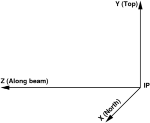
FIG. 1: Tentative coordinate frame of experimental setup.
In this frame photon-hit pixel coordinates (x, y, z) can be easily transformed to the photon diffraction angle θ,
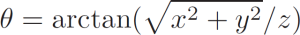 (1)
(1)
Sensor
On the very bottom level of hierarchy structure there should be self-sufficient components of the detector - sensors a.k.a. tiles, segments, pixel arrays/matrix etc. We assume that
- tiles may be of different types even in a single detector,
- all tiles of the same type have identical geometry,
- by design each tile has well defined geometry of pixels which does not need in calibration,
- pixel center (x, y, z) coordinates in each tile can be defined as a look-up table for all pixels,
- each tile is represented in data as a minimal solid block of memory,
- “natural” matrix-style pixel numeration is preferable for simplicity of the tile description but is not necessarily required
For example, CSPAD 2x1 tile pixel geometry is schematically shown in Fig.2.
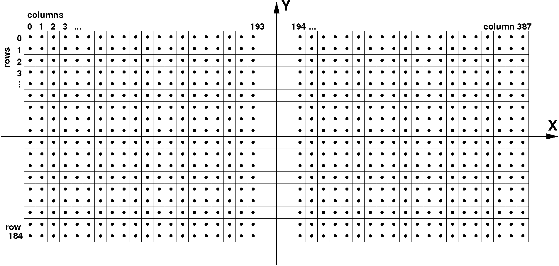
FIG. 2: Coordinate frame of CSPAD 2x1 sensor. Note that a right-handed rule is used for the coordinate system, so the z-axis is coming out of the page. This "native" sensor frame is initially aligned with the global coordinate system; the sensor is then positioned by applying translations and rotations relative to that native frame.
The CSPAD 2x1 tile has
- 185 rows and 388 columns of pixels,
- regular pixel size is 109.92 × 109.92 μm²,
- pixel size in two middle columns (193 and 194) is 274.80 × 109.92 μm².
The pixel index and coordinates in the tile memory block of size 185×388 can be evaluated as
y = k * row + y_offset
x = f(column)
where y coordinate is proportional to the row index, while x coordinate needs to be tabulated as a function of the column index due to the gap in the tile central columns braking matrix uniformity. Detector data record consists of consecutive tile-memory blocks, in accordance with numeration adopted in DAQ. For effective memory management, some of the tile-blocks may be missing due to current detector configuration. Available configuration of the detector tile-blocks should be marked in a configuratiomn bit-mask word in positional order (bit position from lower to higher is associated with the tile number in DAQ).
Child geometry object in the parent frame
Full description of a composite detector (beside top and bottom level hierarchical objects) needs in definition of intermediate objects with their arbitrary location and orientation. Any geometry object coordinate system may have a translation and rotation with respect to the parent object, which can be defined by the 3 vectors in the setup frame as shown in Figure
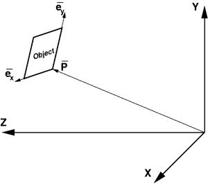
FIG. 3: Child object position in the parent coordinate frame.
where
- P is a translation vector pointing from parent to its child frame origin,
- ex is a unit vector along the child frame x axis,
- ey is a unit vector along the child frame y axis.
Third unit vector ez is assumed to be right-hand triplet component, 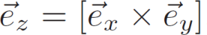 . Components of these three unit vectors form the rotation matrix
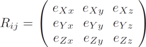 (2)
(2)
where index “j” enumerates unit vectors in the object coordinate frame, and index “i” is an object unit vector component in the parent frame (ex.: eYz is a Y component of the vector ez). Within this definition 3-d pixel coordinate “c” in the object frame can be transformed to the parent coordinate frame “C” using equation
Ci=Rij·cj + Pi. (3)
For practical reason we parametrize rotation matrix Rij in terms of Cardan’s angles R(α, β, γ). We assume that the 3-d rotation matrix R(α, β, γ) is a product of three 2-d rotations
R(α, β, γ) = Rx(α) · Ry(β) · Rz(γ), (4)
around appropriate axes, defined as
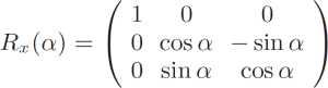
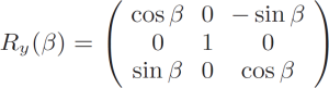
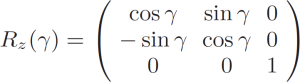 (5)
(5)
This transformation algorithm is implemented in class PSCalib.GeometryObject as discussed below.
Example of composite detector
As an example we show how composite CXI-like CSPAD detector with moving quads can be inscribed in the hierarchical geometry model and how geometry parameters can be retrieved in each level.
- CSPAD 2x1 sensor (Fig. 2) is the low-level object with completely specified geometry of pixels.
- A group of eight cspad 2x1 sensors forms a quad (Fig. 4). Sensors’ positions in the quad can be measured by optical microscope.
- Four quads form a CSPAD detector. In CXI-like CSPAD quads can be moved by the stepping motor. For technical reason this detector can not be measured with optical microscope. Dedicated runs with bright images of test wires, diffraction rings, or Bragg peaks can be used to calibrate relative quad positions. Then, quads’ position variation by the stepping motor can be accounted for once calibrated quads.
- Finally, detector position relative to IP should be accounted (Fig. 6). Detector position and orientation can be measured by the ruler in the hatch for the first approximation. The same dedicated runs with bright images can be used to evaluate precise detector coordinates. Calibration runs with a few detector positions along the beam line can be helpful for full geometry parameters reconstruction.
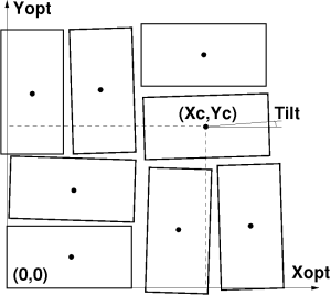
FIG. 4: Example: 2x1 sensors’ positions in the CSPAD quad coordinate frame.
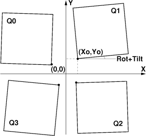
FIG. 5: Example: quads’ positions in the CSPAD detector coordinate frame.
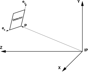
FIG. 6: Example: detector position in the experiment coordinate frame with origin at IP.
Optical measurements
Precise pixel coordinates can be retrieved in a few steps using
- ideal tile design geometry (Fig. 2),
- results of measurements with optical microscope,
- correction of sub-detector elements using dedicated runs.
In this section we describe a procedure of optical measurements, its potential problem, and method to fix it.
Metrology file
Optical measurements with microscope give the most precise information about sensors’ positions in the parent structure. Estimated accuracy of measurements is σRMS ∼ 10μm in x-y plane, and about the same amount in z. Optical measurements provide 3-d coordinates of 4 corners for all tiles in the (sub-)detector in some arbitrary microscope plane which coincides with detector imaging array (tiles) plane within precision of installation.
- Tile corner coordinates do not necessarily coincide with pixel centers or corners.
- Numeration of tiles in optical measurements should not necessarily coincide with their numeration in DAQ, but it should be done in expected order with indication of tile numbers.
- Optical measurements are saved in the xlsx file as a table of x, y, z coordinates for all sensor corners with records like
Tile <#>
Point <#> <X[um]> <Y[um]> <Z[um]>
- Metrology files are produced by the detector group for new or repaired detectors.
Quality check
Measurements with microscope are not automated. Results are manually saved in the metrology file, which may have non-intentional typos. If the number of typos is small they can be tracked down in the quality check and fixed. Quality check of optical measurement may test for each tile:
- equity of opposite sides
- equity of diagonals
- equity of tilt angles for all sides
- tile flatness in 3-d
Report table about all deviations is generated by the python script processing the metrology file. Large deviations exceeding standard precision >3σ(RMS) indicate on problem with measurement. A few corrections are usually applied for each metrology file.
Calibration file
In this section we discuss requirements to the geometry alignment parameters and describe chosen file format.
Hierarchical structure
In the calibration file/table we need to save links between parent and child objects. Tree-like structure assumes that each parental object may have many children and each child object has only one parent. It is easier for each object to keep information about its parent and object location and orientation parameters with respect to the parent, as implemented in class PSCalib.GeometryObject. One fixed length record per object is convenient to keep this information in memory and file as a table. Scan over all objects allows to retrieve all hierarchical links and use them further in recursive processing. This algorithm is implemented in the class PSCalib.GeometryAccess.
Object identification
Composite detector usually consists of similar sub-detectors. In particular, CSPAD consists of four quads, quad consists of eight 2x1 sensors. Sub-detectors of the same type should be treated by the same code. To distinguish between sub-detectors we introduce two variable for each object, name and index. For example, CSPAD quads have an arbitrary symbolic name “QUAD” and indexes from 0 to 3, their children have a symbolic name “CSPAD2X1V1” and indexes from 0 to 7. The name of low level objects, “CSPAD2X1V1”, is used in the factory method PSCalib.SegGeometryStore.Create in order to instantiate associated PSCalib.SegGeometry object. This and all other names are also used to set child-parent relations between objects.
Assumptions about detector geometry
In most cases we deal with planar detectors and we assume that:
- the detector image is produced by a set of tiles,
- all tiles form almost flat (x-y) surface around z=0 within precision of production technology and installation,
- the tile rotation angles in (x-y) are N*90 degrees, where N=0,1,2,or 3, detector local coordinate system is defined
in this plane, as explained below. These assumptions are not necessary for all algorithms. But, in many cases it may be convenient to use small angle approximation or ignore angular misalignment for image mapping between tiles and 2-d image array. For this reason in calibration file we split all angles for rotation and tilt in order to have direct access to the designed and corrected values, respectively.
File format
From metrology file we may evaluate the tile center coordinates as an average over 4 corners. Tilt angles are defined as projected angles of the tile sides on relevant planes. Each angle is evaluated as an averaged angle for 2 sides. The tile location and orientation in the parent frame can be saved in the table record where

- Parent name - name and version of the parent object; all translation and rotation pars are defined w.r.t. parent Cartesian frame
- Parent index - index of the parent object
- Object name - name and version of the object inserted in the parent frame
- Object index - index of the object
- X0, Y0, and Z0 [μm] - object frame origin coordinates in the parent frame
- Rotation X, Y, and Z [degree] - object ideal (design) rotation angle around X, Y, and Z axis of the parent frame, respectively,
- Tilt X, Y, and Z [degree] - tilt angles for correction of the object rotation angles around X, Y, and Z axis of the parent frame, respectively.
First four fields are intended to set parent-to-child relations between geometry objects. Python script in CalibManager reads data from the metrology file and generates the geometry file consisting of records in this format. Thus tabulated geometry parameters allow to
- accommodate parameters from optical measurement,
- update information about sub-detectors later,
- retrieve all hierarchical links.
Result of multiple geometry transformations depends on their order. In coordinate reconstruction algorithms we use particular order for rotations and translations.
Calibration file example
CalibManager under the tabs Geometry / Metrology has a GUI which processes metrology file and generates the calibration file like shown below for CXI-like CSPAD with moving quads
# TITLE      Geometry parameters of CSPAD-CXI
# DATE_TIME  2014-10-03 12:20:44 PDT
# METROLOGY  /reg/neh/home1/dubrovin/LCLS/CSPadMetrologyProc/2014-05-15-CSPAD-CXI-DS1-Metrology-corr.txt
# AUTHOR     dubrovin
# EXPERIMENT Any
# DETECTOR   CSPAD-CXI
# CALIB_TYPE geometry
# COMMENT:01 Table contains the list of geometry parameters for alignment of 2x1 sensors, quads, CSPAD, etc
# COMMENT:02 All translation and rotation pars of the object are defined w.r.t. parent object Cartesian frame
# PARAM:01 PARENT     - name and version of the parent object
# PARAM:02 PARENT_IND - index of the parent object
# PARAM:03 OBJECT     - name and version of the object
# PARAM:04 OBJECT_IND - index of the new object
# PARAM:05 X0         - x-coordinate [um] of the object origin in the parent frame
# PARAM:06 Y0         - y-coordinate [um] of the object origin in the parent frame
# PARAM:07 Z0         - z-coordinate [um] of the object origin in the parent frame
# PARAM:08 ROT_Z      - object design rotation angle [deg] around Z axis of the parent frame
# PARAM:09 ROT_Y      - object design rotation angle [deg] around Y axis of the parent frame
# PARAM:10 ROT_X      - object design rotation angle [deg] around X axis of the parent frame
# PARAM:11 TILT_Z     - object tilt angle [deg] around Z axis of the parent frame
# PARAM:12 TILT_Y     - object tilt angle [deg] around Y axis of the parent frame
# PARAM:13 TILT_X     - object tilt angle [deg] around X axis of the parent frame

# HDR PARENT IND        OBJECT IND    X0[um]  Y0[um]  Z0[um]   ROT-Z ROT-Y ROT-X     TILT-Z   TILT-Y   TILT-X

QUAD:V1        0  SENS2X1:V1     0     21757   33110      51       0     0     0    0.04474 -0.14079 -0.00274
QUAD:V1        0  SENS2X1:V1     1     21769   10457      18       0     0     0    0.01053 -0.11974  0.00000
QUAD:V1        0  SENS2X1:V1     2     33464   68275     -28     270     0     0   -0.01645  0.10414  0.09737
QUAD:V1        0  SENS2X1:V1     3     10769   68299      18     270     0     0   -0.02828  0.02740  0.13418
QUAD:V1        0  SENS2X1:V1     4     68489   56732      71     180     0     0   -0.05128 -0.11309  0.06303
QUAD:V1        0  SENS2X1:V1     5     68561   79628     -20     180     0     0   -0.03552  0.07104 -0.11788
QUAD:V1        0  SENS2X1:V1     6     77637   21754     -15     270     0     0   -0.33657 -0.00821  0.01183
QUAD:V1        0  SENS2X1:V1     7     54810   21558     -54     270     0     0   -0.06315  0.00000  0.00658

QUAD:V1        1  SENS2X1:V1     0     21757   33329     178       0     0     0    0.08883  0.03158 -0.20830
QUAD:V1        1  SENS2X1:V1     1     21773   10446      61       0     0     0   -0.01448  0.04211 -0.24943
QUAD:V1        1  SENS2X1:V1     2     33430   68158     257     270     0     0    0.02698 -0.04660 -0.07370
QUAD:V1        1  SENS2X1:V1     3     10628   68183     247     270     0     0    0.04014 -0.08498 -0.06448
QUAD:V1        1  SENS2X1:V1     4     68349   56949     161     180     0     0   -0.00066 -0.02895  0.05481
QUAD:V1        1  SENS2X1:V1     5     68345   79783     231     180     0     0    0.06843 -0.13948  0.03836
QUAD:V1        1  SENS2X1:V1     6     77454   21811     111     270     0     0    0.05919 -0.06029 -0.11707
QUAD:V1        1  SENS2X1:V1     7     54729   21779     106     270     0     0    0.07632 -0.04933 -0.16580

QUAD:V1        2  SENS2X1:V1     0     21741   33265       0       0     0     0   -0.06053  0.00000  0.00000
QUAD:V1        2  SENS2X1:V1     1     21752   10493       0       0     0     0    0.10132  0.00000  0.00000
QUAD:V1        2  SENS2X1:V1     2     32869   68638       0     270     0     0    0.07036  0.00000  0.00000
QUAD:V1        2  SENS2X1:V1     3     10462   68624       0     270     0     0    0.00658  0.00000  0.00000
QUAD:V1        2  SENS2X1:V1     4     68166   57261       0     180     0     0    0.17894  0.00000  0.00000
QUAD:V1        2  SENS2X1:V1     5     68109   79832       0     180     0     0    0.11972  0.00000  0.00000
QUAD:V1        2  SENS2X1:V1     6     77482   21698       0     270     0     0   -0.02762  0.00000  0.00000
QUAD:V1        2  SENS2X1:V1     7     54709   21779       0     270     0     0    0.02499  0.00000  0.00000

QUAD:V1        3  SENS2X1:V1     0     21730   33098     102       0     0     0    0.09278 -0.05132 -0.27140
QUAD:V1        3  SENS2X1:V1     1     21755   10477      40       0     0     0    0.06580 -0.02369 -0.32612
QUAD:V1        3  SENS2X1:V1     2     33193   68452     272     270     0     0    0.34083 -0.02192 -0.18687
QUAD:V1        3  SENS2X1:V1     3     10904   68416     270     270     0     0    0.01645  0.00823 -0.15397
QUAD:V1        3  SENS2X1:V1     4     68570   56923     194     180     0     0    0.12435  0.06974  0.07401
QUAD:V1        3  SENS2X1:V1     5     68456   79666     246     180     0     0    0.20857  0.04737  0.12882
QUAD:V1        3  SENS2X1:V1     6     77425   21681      60     270     0     0    0.05264  0.00274 -0.30004
QUAD:V1        3  SENS2X1:V1     7     54648   21761     118     270     0     0    0.01645 -0.00822 -0.22107

CSPAD:V1       0  QUAD:V1        0     -4500   -4500       0      90     0     0    0.00000  0.00000  0.00000
CSPAD:V1       0  QUAD:V1        1     -4500    4500       0       0     0     0    0.00000  0.00000  0.00000
CSPAD:V1       0  QUAD:V1        2      4500    4500       0     270     0     0    0.00000  0.00000  0.00000
CSPAD:V1       0  QUAD:V1        3      4500   -4500       0     180     0     0    0.00000  0.00000  0.00000
All lines started with hash “#” are comments, which are also accessible through the program interface as a dictionary. XPP-like CSPAD with all sensors attached to the same plate is measured as a single detector. Its content part omits quads
# TITLE      Geometry parameters of CSPAD-XPP
# METROLOGY  /reg/neh/home1/dubrovin/LCLS/CSPadMetrologyProc/2013-10-09-CSPAD-XPP-Metrology.txt
...

# HDR PARENT IND        OBJECT IND    X0[um]  Y0[um]  Z0[um]   ROT-Z ROT-Y ROT-X     TILT-Z   TILT-Y   TILT-X
CSPAD:V2       0  SENS2X1:V1     0     51621  112683     153      90     0     0    0.48292  0.00000  0.00263
CSPAD:V2       0  SENS2X1:V1     1     74168  112907     135      90     0     0    0.48886 -0.05755  0.01316
CSPAD:V2       0  SENS2X1:V1     2     16366  124137     107       0     0     0    0.32370  0.00395 -0.01096
CSPAD:V2       0  SENS2X1:V1     3     16415  101350     185       0     0     0    0.15130  0.09867 -0.29055
CSPAD:V2       0  SENS2X1:V1     4     27786  159233     123     270     0     0    0.24474 -0.03015  0.03948
CSPAD:V2       0  SENS2X1:V1     5      4845  159260     106     270     0     0    0.05987 -0.04659  0.01053
CSPAD:V2       0  SENS2X1:V1     6     62758  168631     132       0     0     0    0.44940  0.02895 -0.00548
CSPAD:V2       0  SENS2X1:V1     7     62881  145851     137       0     0     0    0.20068  0.03553 -0.03015
CSPAD:V2       0  SENS2X1:V1     8    107098  129494     165       0     0     0    0.01316  0.01184 -0.02742
CSPAD:V2       0  SENS2X1:V1     9    107067  106699     152       0     0     0   -0.15924 -0.01316 -0.05208
CSPAD:V2       0  SENS2X1:V1    10    118871  164660     152     270     0     0    0.11249 -0.02193  0.04078
CSPAD:V2       0  SENS2X1:V1    11     95879  164632     143     270     0     0   -0.07632 -0.05757  0.03158
CSPAD:V2       0  SENS2X1:V1    12    153905  153051     158     180     0     0   -0.03026  0.00000 -0.04385
CSPAD:V2       0  SENS2X1:V1    13    153838  175841     140     180     0     0   -0.03947 -0.01973 -0.16719
CSPAD:V2       0  SENS2X1:V1    14    163149  117980     156     270     0     0   -0.17500 -0.04385 -0.00526
CSPAD:V2       0  SENS2X1:V1    15    140287  117936     153     270     0     0    0.00000 -0.02741 -0.00790
CSPAD:V2       0  SENS2X1:V1    16    123905   73726     133     270     0     0    0.00263 -0.00548 -0.00921
CSPAD:V2       0  SENS2X1:V1    17    101282   73699     130     270     0     0    0.20725 -0.02740 -0.03948
CSPAD:V2       0  SENS2X1:V1    18    159023   62203     142     180     0     0   -0.05461 -0.00263 -0.03562
CSPAD:V2       0  SENS2X1:V1    19    159024   84885     136     180     0     0   -0.08026  0.01579 -0.06576
CSPAD:V2       0  SENS2X1:V1    20    147998   26847     106      90     0     0    0.03158 -0.08219  0.08947
CSPAD:V2       0  SENS2X1:V1    21    170404   26856      96      90     0     0   -0.07893 -0.00822  0.06972
CSPAD:V2       0  SENS2X1:V1    22    112701   17748      97     180     0     0    0.26908 -0.02500 -0.00548
CSPAD:V2       0  SENS2X1:V1    23    112640   40586     100     180     0     0    0.03685 -0.01448  0.03836
CSPAD:V2       0  SENS2X1:V1    24     68448   57015     119     180     0     0    0.27835 -0.02501  0.09319
CSPAD:V2       0  SENS2X1:V1    25     68292   79701     120     180     0     0    0.37440 -0.03290 -0.04112
CSPAD:V2       0  SENS2X1:V1    26     56919   21965      69      90     0     0    0.18024 -0.06578  0.07894
CSPAD:V2       0  SENS2X1:V1    27     79497   22002      67      90     0     0    0.12040 -0.02740  0.09211
CSPAD:V2       0  SENS2X1:V1    28     21658   33119      72       0     0     0    0.27240  0.03553 -0.12332
CSPAD:V2       0  SENS2X1:V1    29     21748   10489      28       0     0     0    0.09805  0.03027 -0.07946
CSPAD:V2       0  SENS2X1:V1    30     12357   68156      97      90     0     0    0.20919  0.03562  0.05789
CSPAD:V2       0  SENS2X1:V1    31     35247   68250      89      90     0     0    0.09144 -0.04109  0.02368
Content of CSPAD2x2 geometry file consist of data for two sensors only:
# TITLE      Geometry parameters of CSPAD2X2
# METROLOGY  /reg/neh/home1/dubrovin/LCLS/CSPad2x2Metrology/CSPad2x2/2014-04-25-CSPAD2X2-3-MEC-Metrology.txt
...

# HDR PARENT IND        OBJECT IND    X0[um]  Y0[um]  Z0[um]   ROT-Z ROT-Y ROT-X     TILT-Z   TILT-Y   TILT-X

CSPAD2X1:V1    0  SENS2X1:V1     0     21848   10490       6     180     0     0   -0.00197 -0.01049  0.03004
CSPAD2X1:V1    0  SENS2X1:V1     1     21943   33908       4     180     0     0   -0.16127 -0.00262 -0.01639
If the detector pixel coordinates should be presented relative to IP or other setup component, have an offset or flipped around axis one more line must to be added, for example
# HDR PARENT IND        OBJECT IND    X0[um]  Y0[um]  Z0[um]   ROT-Z ROT-Y ROT-X     TILT-Z   TILT-Y   TILT-X
SETUP-IP       0   CSPAD2X2:V1   0      -100     200 1000000       0   180     0          0        0        0
Interface implementation
Program interface to the detector geometry parameters consists of a few modules with the same names up to extensions for C++ and Python in the PSCalib package. Sensor geometry:
- PSCalib.SegGeometry - abstract interface for sensor pixels geometry description.
- PSCalib.SegGeometryCspad2x1V1 - implementation of interface for CSPAD 2x1 sensor of version V1.
- PSCalib.SegGeometryStore - static factory method for all available sensor geometry descriptors.
Hierarchical model:
- PSCalib.GeometryObject - class to support one object/node in hierarchical structure.
- PSCalib.GeometryAccess - class to support hierarchical structure and access to the geometry parameters.
C++ program interface description with examples is available in Doxygen documentation. Below we consider Python interface only.
Access to sensor geometry information
Generic program interface to the sensors’ ideal geometry is presented by the abstract class PSCalib.SegGeometry. It declares methods returning number of pixels, rows, columns, pixel size, area, center coordinates relative to sensor coordinate frame, as listed below.
def print_seg_info(self, pbits=0) :
""" Prints segment info for selected bits"""
def size(self) :
""" Returns segment size - total number of pixels in segment"""
def rows(self) :
""" Returns number of rows in segment"""
def cols(self) :
""" Returns number of cols in segment"""
def shape(self) :
""" Returns shape of the segment [rows, cols]"""
def pixel_scale_size(self) :
""" Returns pixel size in um for indexing"""
def pixel_area_array(self) :
""" Returns array of pixel relative areas of shape=[rows, cols]"""
def pixel_size_array(self, axis) :
""" Returns array of pixel size in um for AXIS"""
def pixel_coord_array(self, axis) :
""" Returns pointer to the array of segment pixel coordinates in um for AXIS"""
def pixel_coord_min(self, axis) :
""" Returns minimal value in the array of segment pixel coordinates in um for AXIS"""
def pixel_coord_max(self, axis) :
""" Returns maximal value in the array of segment pixel coordinates in um for AXIS"""
def pixel_mask_array(self, mbits) :
""" Returns array of masked pixels which content depends on bontrol bitword mbits"""
Currently this abstract interface has the only implementation for CSPAD2x1 in the class PSCalib.SegGeometryCspad2x1V1. Other versions of CSPAD2x1, ePix, pnccd, etc. sensors can be added later. Static factory method Create in class PSCalib.SegGeometryStore allows to access any sensor geometry information by the detector independent way. For example, pixel x-, y-, and z-coordinate arrays can be directly retrieved from class PSCalib.SegGeometryCspad2x1V1:
from PSCalib.SegGeometryCspad2x1V1 import cspad2x1_one

xarr, yarr, zarr = cspad2x1_one.pixel_coord_array()
or using generic access method through the factory method:
from PSCalib.SegGeometryStore import sgs

sg = sgs.Create(’SENS2X1:V1’, pbits=0377)
xarr, yarr, zarr = sg.pixel_coord_array()
return the same x-, y-, and z-coordinate arrays of shape=[185,388].
This interface is used internally in the geometry service modules and, until it is absolutely necessary, should not be used directly. Doxygen/Sphinx documentation for C++/Python modules is available in References.
Pixel coordinates transformation
Child geometry object pixel coordinates are transformed to the parent frame pixel coordinates in accordance with Eqn 3. We use rotation matrix expressed in terms of cosines and sines of rotation angles as shown in Eqs. 4-5 First we apply rotations around z, y, and x axes then translation. Note, that order of operations is important. This transformation algorithm is implemented in the class PSCalib.GeometryObject. For example, in Python module PSCalib.GeometryObject.py all transformations of pixel coordinate arrays are presented by the code
#file: pyimgalgos/src/GeometryObject.py

def rotation(X, Y, C, S) :
    Xrot = X*C - Y*S
    Yrot = Y*C + X*S
    return Xrot, Yrot

class GeometryObject :
    ...
    def transform_geo_coord_arrays(self, X, Y, Z) :
        ...
	    # define Cx, Cy, Cz, Sx, Sy, Sz - cosines and sines of rotation + tilt angles
        ...
        X1, Y1 = rotation(X,  Y,  Cz, Sz)
        Z2, X2 = rotation(Z,  X1, Cy, Sy)
        Y3, Z3 = rotation(Y1, Z2, Cx, Sx)

        Zt = Z3 + self.z0
        Yt = Y3 + self.y0
        Xt = X2 + self.x0

        return Xt, Yt, Zt
Detector geometry access interface
Public methods of the class PSCalib.GeometryAccess:
def __init__(self, path, pbits=0) :
"""Constructor of the class"""
def get_pixel_coords(self, oname=None, oindex=0) :
"""Returns three pixel X,Y,Z coordinate arrays for top or specified geometry object"""
def get_pixel_areas(self, oname=None, oindex=0) :
"""Returns pixel areas array for top or specified geometry object"""
def get_pixel_mask(self, oname=None, oindex=0, mbits=0377) :
"""Returns pixel mask array for top or specified geometry object.
mbits =+1 - mask edges
       +2 - two wide-pixel central columns
       +4 - non-bounded pixels
       +8 - neighbours of non-bounded pixels"""
def get_pixel_scale_size(self, oname=None, oindex=0) :
"""Returns pixel scale size for top or specified geometry object"""
def get_dict_of_comments(self) :
"""Returns dictionary of comments"""
def set_geo_pars(self, oname=None, oindex=0, x0=0, y0=0, z0=0, rot_z=0, rot_y=0, rot_x=0, tilt_z=0, tilt_y=0, tilt_x=0) :
"""Sets geometry parameters for specified or top geometry object"""
def move_geo(self, oname=None, oindex=0, dx=0, dy=0, dz=0) :
"""Moves specified or top geometry object by dx, dy, dz"""
def tilt_geo(self, oname=None, oindex=0, dt_x=0, dt_y=0, dt_z=0) :
"""Tilts specified or top geometry object by dt_x, dt_y, dt_z"""
def print_list_of_geos(self) :
def print_list_of_geos_children(self) :
def print_comments_from_dict(self) :
def print_pixel_coords(self, oname=None, oindex=0) :
"""Partial print of pixel coordinate X,Y,Z arrays for selected or top(by default) geo"""
def get_pixel_coord_indexes(self, oname=None, oindex=0, pix_scale_size_um=None, xy0_off_pix=None) :
"""Returns three pixel X,Y,Z coordinate index arrays for top or specified geometry object"""
def set_print_bits(self, pbits=0) :
""" Sets printout control bitword"""
def set_print_bits(self, pbits=0) :
""" Sets printout control bitword"""
def get_psf(self) :
"""Returns array of vectors in TJ format (psf stands for position-slow-fast vectors)"""
def print_psf(self) :
""" Gets and prints psf array for test purpose"""

# private methods, which may be useful:
def get_geo(self, oname, oindex) :
"""Returns specified geometry object"""
def get_top_geo(self) :
"""Returns top geometry object"""

# global method:
def img_from_pixel_arrays(iX, iY, W=None, dtype=np.float32) :
"""Returns image from iX, iY coordinate index arrays and associated weights W"""
For example:
from PSCalib.GeometryAccess import *
fname_geometry = ’<path>/geometry/0-end.data’
geometry = GeometryAccess(fname_geometry, 0377)

pix_size = geometry.get_pixel_scale_size()
X, Y, Z = geometry.get_pixel_coords(’QUAD:V1’, 1) # for quad
X, Y, Z = geometry.get_pixel_coords() # for top object (CSPAD)
iX, iY = geometry.get_pixel_coord_indexes(’QUAD:V1’, 1, pix_scale_size_um=None, xy0_off_pix=None) # for quad
iX, iY = geometry.get_pixel_coord_indexes(xy0_off_pix=(1000, 1000)) # for top object (CSPAD)
img = img_from_pixel_arrays(iX,iY,W=<intensity-array>)
img = img_from_pixel_arrays(iX,iY) # Image of 0/1 for fake/real pixels
arr = geometry.get_pixel_mask(’QUAD:V1’, 1, 1+2+4+8)
arr.shape = (8,185,388)

dict_comm = geometry.get_dict_of_comments()
d = geometry.get_dict_of_comments()
print "d[’DATE_TIME’] = %s" % d[’DATE_TIME’]
Geometry File Format Conversion
crystfel/cheetah/psana
Mikhail Dubrovin has created geometry-conversion scripts. Documentation can be found here: Geometry converter between psana and CrystFEL.
TJ Lane has created geometry-conversion scripts. These were originally in github (https://github.com/LinacCoherentLightSource/psgeom) but have been moved into psana. The methods can be accessed in python but an easier to use wrapper script called "geoconv" has been created. Use "geoconv --help" to see the current syntax.
cctbx/psana
Cctbx.xfel conversion instruction can be found here: http://viper.lbl.gov/cctbx.xfel/index.php/Cxi02416_calibration. Use the following command to convert cbf to psana format:
cxi.cbfheader2slaccalib
There's a command to go from psana format to cctbx, it's not documented above but Aaron Brewster says it is
cxi.slaccalib2cbfheader
Summary
Pixel detector geometry generic parameterization presented in this note is implemented in LCLS analysis software releases since ana-0.13.N. Both C++ and Python interfaces are available.
References
- geometry.pdf - this note in PDF format
- Euler angles, Tait–Bryan angles, nautical angles, Cardan angles etc.
- Autogenerated docs - API description for C++ and Python code
- Python API:
- PSCalib.SegGeometry - abstract interface for sensor pixels geometry description.
- PSCalib.SegGeometryCspad2x1V1 - implementation of interface for CSPAD 2x1 sensor of version V1.
- PSCalib.SegGeometryStore - static factory method for all available sensor geometry descriptors.
- PSCalib.GeometryObject - class to support one object/node in hierarchical structure.
- PSCalib.GeometryAccess - class to support hierarchical structure and access to the geometry parameters.
- LAMP_User_Manual.pdf (useful for determining geometry orientation associated with pnCCD readout order (see table 3))
- Detector alignment tool
- Calibration Management Tool
Overview
Content Tools