Page History
...
- Boom! An edge! The edge moves back and forth on the camera screen depending on the relative time delay between the laser and x-rays.
- Wiggles. The nearly-constant sine-like wave is undesirable background due to an etalon effect inside the TT target. Good analysis will remove it (read on). The etalon is especially bad here – it's amplitude and frequency will depend on the target.
- Limited dynamic range. The edge is big with respect to the camera. The TT has about ~1 ps of dynamic range in a given physical setup. That's fine, because the typical jitter in arrival times between x-rays and laser at LCLS is much less than that. Also, the white light pulse is only ~1 ps long! To change the delay "window" the TT is looking at, a delay stage is used to move the white light in time to keep it matched to the x-rays. It is important, however, to keep an eye on the TT signal and make sure it doesn't drift off the camera!
- Read right-to-left. In this image, the white light arriving before the x-rays is to the right, and following it in time takes us to the left. So time is right to left. Just keeping you on your toes.
Default Analysis: DAQ
TimeTool Timetool results can be computed by the DAQ while data is being recorded and written directly into the .xtc files. This is almost always done. The DAQ's processing algorithm is quite good, and most users can employ those results without modification. This section will detail how the DAQ's algorithm works, access those results, assess their quality. Even if you are going to eventually implement your own solution, understanding how this analysis works will be useful. Further, in almost all cases, the DAQ results are good enough for online monitoring of the experiment.
How it works
The goal is to find the edge position, the imprint of the x-rays on the white light pulse, along the x-axis of the OPAL camera. To do this, the DAQ uses a matched filter – that means the filter looks just like the expected signal (an edge) and is "translated" across the signal, looking for the x-position of maximal matchy match. More technically: the filter is convoluted with the signal, and the convolution has a peak. That peak is identified as the edge "position" and gives your time signal. Here is an example of a TT trace (top) and the resulting convolution (bottom) used to locate the edge:
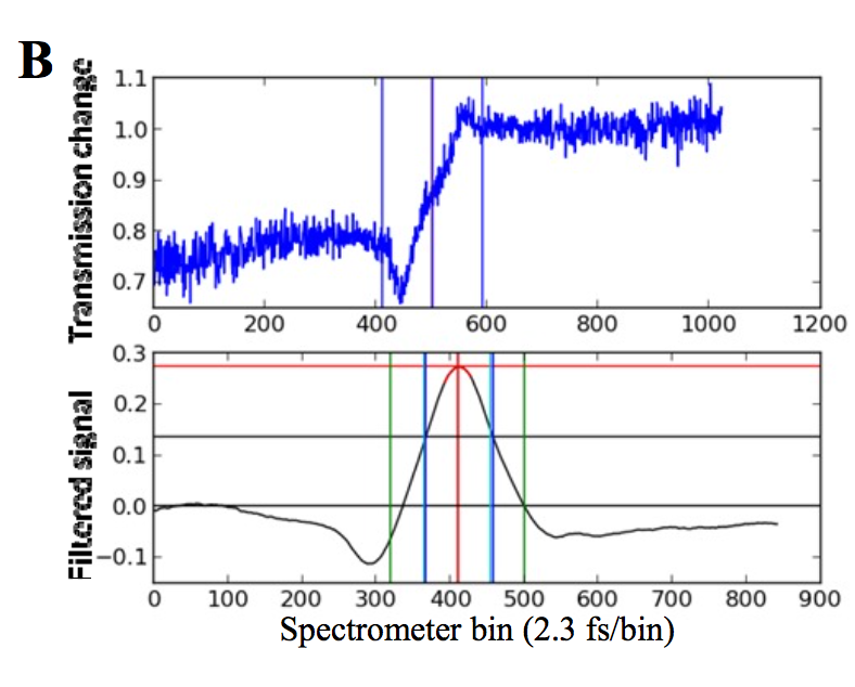
The FWHM of the convolution and it's amplitude are good indicators of how well this worked, and are also reported.
The astute reader will notice that this trace has no etalon wiggles. That is because it has been cleaned up by subtracting an x-ray off shot (BYKICK). Those events have the same etalon effect, but no edge – subtracting them removes the etalon. That's a good thing, because the etalon wiggles would have given this method a little trouble if they were big in amplitude.
So, to summarize, here is what the DAQ analysis code does:
- Extract the TT trace using an ROI + projection
- Subtract the most recent x-ray off (BYKICK) trace
- Convolve the trace with a filter
- Report the position, amplitude, FWHM of the resulting peak
The reported position will be in PIXELS. That is not so useful! To convert to femtoseconds, we need to calibrate the TT.
How to get the results
, or after data has been recorded. In AMO/XPP the time tool analysis is done by the DAQ while data is being recorded. Results can be accessed using the following epics-variables names:
| TTSPEC:FLTPOS | the position of the edge, in pixels |
| TTSPEC:AMPL |
...
| amplitude of biggest edge found by the filter |
...
| TTSPEC:FLTPOSFWHM | the FWHM of the edge, in pixels |
| TTSPEC:AMPLNXT |
...
| amplitude of second-biggest edge found by the filter |
...
| , good for rejecting bad fits |
| TTSPEC: |
...
| REFAMPL | amplitude of the background "reference" which is subtracted before running the filter algorithm, good for rejecting bad fits |
| TTSPEC:FLTPOS_PS |
...
| the position of the edge, in picoseconds, but requires correct calibration constants be put in the DAQ when data is acquired |
...
| . Few people do this. So be wary. |
These are usually pre-pended by the hutch, so e.g. at XPP they will be "XPP:TTSPEC:FLTPOS". The TT camera (an OPAL) should also be in the datastream.
Here is an example of how to get these values from psana
| Code Block | ||||||||
|---|---|---|---|---|---|---|---|---|
| ||||||||
import psana

ds = psana.MPIDataSource('exp=cxij8816:run=221')

evr       = psana.Detector('NoDetector.0:Evr.0')
tt_camera = psana.Detector('Timetool')
tt_pos    = psana.Detector('CXI:TTSPEC:FLTPOS')
tt_amp    = psana.Detector('CXI:TTSPEC:AMPL')
tt_fwhm   = psana.Detector('CXI:TTSPEC:FLTPOSFWHM')

for i,evt in enumerate(ds.events()):
    tt_img = tt_camera.raw(evt)
# <...> |
How to know it did the right thing
Cool! OK, so how do you now if it worked?
| Tip | ||
|---|---|---|
| ||
If you make a plot of the measured timetool delay it is quite noisy (e.g. the laser delay vs. the measured filter position, TTSPEC:FLTPOS, while keeping the TT stage stationary). There are many outliers. This can be greatly cleaned up by filtering based on the TT peak. I (TJ, <tjlane@slac.stanford.edu>) have found the following "vetos" on the data to work well, though they are quite conservative (throw away a decent amount of data). That said they should greatly clean up the TT response and has let me proceed in a "blind" fashion: Require: tt_amp [TTSPEC:AMPL] > 0.05 AND 50.0 < tt_fwhm [TTSPEC:FLTPOSFWHM]< 300.0 This was selected based on one experiment (cxii2415, run 65) and cross-validated against another (cxij8816, run 69). |
Always Calibrate! Why and How.
Rolling Your Own
Overview
Content Tools