This is an unmodified version of exercise 4 from the 2005 Cern School of Computing. With some cleanup it could be made into a introduction to SLIC/LCDD. The code for the exercise is attached.
Simulation, Visualization, and Analysis
...
Although SLIC can be used to set up arbitrarily complex detector geometries this typically involves more work than we have time for in this exercise, so instead you will set up a simple test calorimeter, corresponding to that described in this NIMA 487 (2002) 291-307. The detector you will set up consists of 18 layers, each 1m square in the xy direction, with 8mm of lead followed by 2mm of plastic scintillator in the z direction. The scintillator is read out using photomultipliers, and thus represent the "sensitive" part of the calorimeter. We will simulate the effect of firing electrons at various energies into the front of the calorimeter. The goal of the exercise is to write out a file containing the simulated "hits" in the sensitive layers, and then to analyze this file to determine the energy resolution of the calorimeter for various electron energies.
...
| Tip | ||
|---|---|---|
| ||
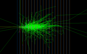
In the event display above you will only see the trajectory of the initial particle fired by the GPS gun into the calorimeter. It will stop somewhere near the entrance to the calorimeter, as it interacts and forms secondary particles. Since a shower consists of many secondary particles we do not normally keep the trajectories of all these particles, as they increase the size of the output file, and slow down Geant4. You can change this behaviour by setting store_secondaries=true in the DetectorRegion in your ecal.lcdd file, in which case you would see something like this: |

...
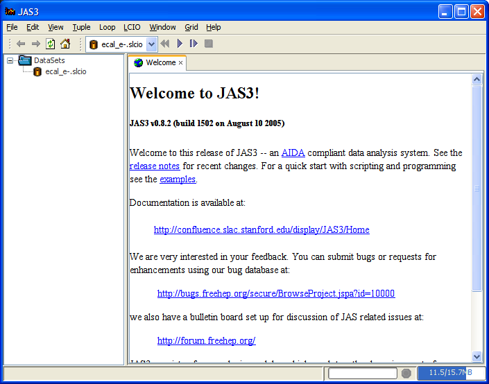
You can now close the plugin manager and open the data file (which should be called ecal-e-.slcio) using the "File", "Open File" menu item in the JAS3 menu bar. Once you open the file it should appear in the JAS3 tree, and a new item should appear in the JAS3 toolbar, allowing you to step through events. You can check that the file contents looks reasonable using two tools, the LCIO Event Browser, and the WIRED4 event display.

To use the Event Browser step to the first event (using the  button in the tool bar) and then from the LCIO menu select "Event Browser".
...
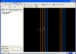
Now you should be able to select "File", "New", "WIRED4 View" in JAS3 and view the event. You should be able to step through different events to see how they look.
Analyzing the Data Files using JAS3
...
- Open the file using the "File", "Open File" menu item. The file will open in the JAS built-in editor (but you can use a different editor if you like to edit the file).
- Compile the file using the JAS compiler. The easiest way is to right-click on the JAS built-in editor and choose "Compile" from the popup menu.
- Load the program into memory using the "Load" item on the JAS popup menu.
- If you have not already done so, open the ecal_e-.slcio file using the "File", "Open File" menu item. If you have already opened the file make sure you are at the beginning of the file by choosing the "Rewind" item from the "Loop" menu.
- Now analyze the data by choosing "Go" from the "Loop" menu. The data will be read, and each event in turn will be passed to the recordSupplied() method of your analysis code. As histograms are created and filled they will appear in the JAS3 tree. You can double-click on the icons corresponding to histograms in the tree to view them, or use the popup-menu on the JAS3 tree to arrange multiple plots on the page.

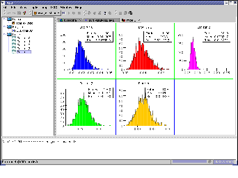
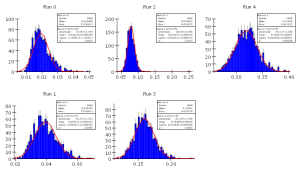
After you have analyzed all of the events you should have one histogram of total energy deposited in the calorimeter for each electron energy you generated with Geant4. Your plots should look something like this:
...
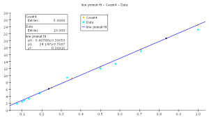
The final step in the analysis is to perform a fit to each energy distribution, to compute the measured energy resolution at each incident electron energy. We will fit a Gaussian function to each of the histograms we produced to compute the mean and sigma of the distribution, and we can then compute the energy resolution as sigma/mean. To compare to the published data we can then produce a plot of energy resolution (in percent) vs sqrt(electron energy), and compare to the published data tabulated below.
You have the choice of performing this part of the analysis using either Java, Python or Pnuts (a simple to learn Java-like scripting language). We have provided templates for the solution in each language in the ~//ex4 directory:
...
You should produce plots which look something like the following plots:


Additional Exercises
...