Background
Josh Lande recently ran some consistency tests comparing the Monte Carlo point source parameters to the values fit by binned likelihood for point sources. For the spacecraft data, he used a one-day interval of the idealized +/-50 deg rocking provided by gtobssim. For one location on the sky, location 0: (RA, Dec) = (176.31, 44.28), the fitted flux in the 0.1-100 GeV band was too high relative to the MC value by ~8%, whereas at location 1: (RA, Dec) =
...
(-176.31,
...
-44.28),
...
the
...
disparity
...
appeared
...
negligible.
...
For
...
such
...
a
...
short
...
time
...
scale
...
(1
...
day),
...
these
...
two
...
sky
...
locations
...
have
...
very
...
different
...
off-axis
...
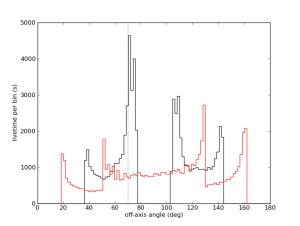
profiles.
...
Here
...
are
...
histograms
...
of
...
the
...
livetime
...
as
...
a
...
function
...
of
...
off-axis
...
angle
...
for
...
the
...
two
...
locations.
...
The
...
black
...
histogram
...
corresponds
...
to
...
location
...
0,
...
and
...
the
...
red
...
corresponds
...
to
...
location 1.
Diagnosis
The bug lay in the code that computes the exposure averaged PSF. This is given by
| Latex |
|---|
1. !off_axis_histograms.png|thumbnail! h3. Diagnosis The bug lay in the code that computes the exposure averaged PSF. This is given by {latex} \newcommand{\e}{\varepsilon} \newcommand{\Int}{{\displaystyle \int}} \begin{eqnarray} P(\psi, \e) &=& \frac{\Int dt P(\psi, \e, \theta) A(\e, \theta)} {\Int dt A(\e, \theta)}\\ &=& \frac{\Int d\theta P(\psi, \e, \theta(t)) A(\e, \theta(t))|\partial\theta/\partial t|^{-1}} {\Int d\theta A(\e, \theta(t)) |\partial\theta/\partial t|^{-1}} \end{eqnarray} {latex} Here {latex}$P${latex} and {latex}$A${latex} are the PSF and effective area, respectively, and {latex} |
Here
| Latex |
|---|
$P$ |
| Latex |
|---|
$A$ |
| Latex |
|---|
$\theta=\theta(t)$ |
...
| Latex |
|---|
$P$ |
| Latex |
|---|
$A$ |
| Latex |
|---|
$\psi$ |
| Latex |
|---|
$\varepsilon$ |
In ST-09-27-01
...
and
...
earlier,
...
there
...
is
...
a
...
cutoff
...
at
...
theta=70
...
deg
...
for
...
the
...
mean
...
PSF
...
calculation.
...
The
...
original
...
reason
...
for
...
this
...
cutoff
...
is
...
unclear,
...
but
...
it
...
was
...
probably
...
motivated
...
by
...
some
...
poor
...
behavior
...
of
...
the
...
PSF
...
at
...
large
...
theta
...
angles
...
for
...
an
...
early
...
version
...
of
...
the
...
IRFs.
...
As
...
far
...
as
...
the
...
shape
...
of
...
the
...
PSF
...
is
...
concerned,
...
this
...
truncation
...
does
...
not
...
have
...
a
...
significant
...
effect.
...
As
...
part
...
of
...
some
...
recent
...
refactoring,
...
this
...
truncation
...
was
...
removed
...
in
...
Likelihood-17-22-04
...
(22
...
Feb
...
2012).
...
Unfortunately,
...
I
...
had
...
thought
...
that
...
the
...
truncation
...
only
...
affected
...
the
...
PSF
...
shape
...
calculation.
...
In
...
fact,
...
for
...
point
...
sources,
...
the
...
binned
...
analysis
...
code
...
has
...
been
...
using
...
the
...
exposure
...
calculation
...
in
...
the
...
denominator
...
of
...
the
...
mean
...
PSF
...
expression
...
for
...
computing
...
the
...
model
...
counts
...
rather
...
than
...
using
...
the
...
exposure
...
from
...
the
...
binned
...
exposure
...
map.
...
Hence,
...
all
...
point
...
source
...
fits
...
will
...
be
...
affected
...
by
...
this
...
truncation.
...
For
...
location
...
0
...
(black
...
histogram
...
in
...
above
...
figure),
...
a
...
significant
...
fraction
...
of
...
its
...
time
...
is
...
spent
...
just
...
beyond
...
the
...
theta=70
...
deg
...
cutoff.
...
This
...
is
...
the
...
cause
...
of
...
the
...
8%
...
disparity
...
that
...
Josh
...
found
...
in
...
his
...
tests.
...
Effects
One can estimate the impact of the theta=70
...
deg
...
cutoff
...
by
...
running
...
gtexpcube2
...
with
...
the
...
option
...
thmax=180
...
in
...
the
...
nominal
...
case
...
(this
...
is
...
the
...
default)
...
and
...
thmax=70
...
in
...
the
...
truncation
...
case.
...
Assuming
...
a
...
photon
...
index
...
of
...
-2,
...
which
...
Josh
...
used
...
in
...
his
...
gtobssim
...
runs,
...
one
...
can
...
estimate
...
the
...
expected
...
fractional
...
offset
...
in
...
measured
...
flux
...
(Fmeas)
...
relative
...
to
...
the
...
MC
...
value
...
(Fmc),
...
(Fmeas
...
-
...
Fmc)/Fmc,
...
using
...
the
...
spectrally
...
weighted
...
exposures,
...
exposure
...
| Latex |
|---|
...
$= \left.\int \varepsilon^{-2} A(\varepsilon, \theta(t)) dt d\varepsilon\right/\int \varepsilon^{-2} d\varepsilon$ |
...
...
and
...
computing
...
(exposure180
...
-
...
exposure70)/exposure70.
...
For
...
the
...
one-day
...
simulation,
...
here
...
is
...
a
...
map
...
of
...
the
...
estimated
...
fractional
...
offset
...
in
...
Galactic
...
coordinates:
...
- One
...
- day
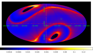
The green point near the Northern Galactic pole is location 0 and has a fractional flux offset of 8%, and the green point nearer the Galactic plane has flux offset of 1.5%. The peak offsets can be has high as 16.3%.
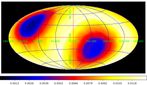
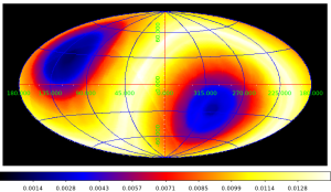
On longer time scales, these offsets are considerably smaller. Here are maps for the 18 month and 2 year livetime cubes used by the catalog group for 2FGL:
- 18 months (/afs/slac/g/glast/groups/catalog/P6_V8_DIFFUSE/ltcube_18months_rock52.fits)
...
- 2 years (/afs/slac/g/glast/groups/catalog/P6_V8_DIFFUSE/ltcube_2years_rock52.fits)
...
I've
...
computed
...
livetime
...
cubes
...
for
...
30
...
day
...
intervals
...
and
...
have
...
estimated
...
the
...
fractional
...
offset
...
as
...
a
...
function
...
of
...
time
...
for
...
the
...
Vela,
...
Crab,
...
and
...
Geminga
...
pulsars.
...
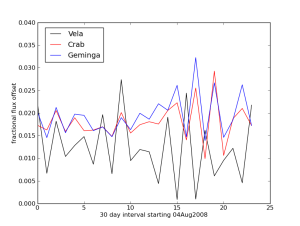
There is a DC offset of about 1.5%
...
and
...
an
...
additional
...
dispersion
...
of
...
about
...
the
...
same
...
size.
...
NB:
...
These
...
estimates
...
assume
...
a
...
power-law
...
spectrum
...
with
...
photon
...
index
...
-2
...
over
...
the
...
entire
...
integration
...
range
...
0.1-100
...
GeV.
...