...

Cool! OK, so how do you now if it worked? Here are a number of things to check:

1. Plot some TT traces with the edge position on top of them, and make sure the edge found is reasonable.
2. Look at a "jitter histogram", that is the distribution of edge positions found, for a set time delay. The distribution should be approximately Gaussian. Not perfectly. But it should not be multi-modal.
3. Do pairwise correlation plots between TTSPEC:FLTPOS / TTSPEC:AMPL / TTSPEC:FLTPOSFWHM, and ensure that you don't see anything "weird". They should form nice blobs – maybe not perfectly Gaussian, but without big outliers, periodic behavior, or "streaks".
4. Analyze a calibration run, where you change the delay in a known fashion, and make sure your analysis matches that known delay (see next section).
5. The gold standard: do your full data analysis and look for weirdness. Physics can be quite sensitive to issues! But it can often be difficult to trouble shoot this way, as many things could have caused your experiment to screw up.

Outliers in the timetool analysis are common, and most people typically throw away shots that fall outside obvious "safe" regions. That is totally normal, and typically will not skew your results.

Always Calibrate! Why and How.

As previously mentioned, the timetool trace edge is found and reported in pixels along the OPAL camera (e.g. arbitrary spatial units), and must be converted into a time delay (in femtoseconds). Because the TT response is a function of geometry, and that geometry can change even during an experiment due to thermal expansion, changing laser alignment, different TT targets, etc, frequent calibration is recommended. A good baseline recommendation is to do it once per shift, and then again if something affecting the TT changes.

To calibrate, we drive the timetool delay stage (for the white light) while keeping the nominal delay between the x-rays and laser constant. This causes the edge to transverse the camera, going from one end to the other, as the white light delay changes due to the changing propagation length. Because we know the speed of light, we can figure out what the change in time delay was, and use that known value to calibrate how much the edge moves (in pixels) for a given time delay change.

Two practicalities to remember:

1. There is inherent jitter in the arrival time between x-rays and laser (remember, this is why we need the TT!). So to do this calibration we have to average out this jitter across many shots. The jitter is typically roughly Gaussian, so this works.
2. The delay-to-edge conversion is not generally perfectly linear. In common use at LCLS is a 2nd order polynomial fit (phenomenological) which seems to work great.

Here's a typical calibration result from CXI, with vetos applied:

Image Added

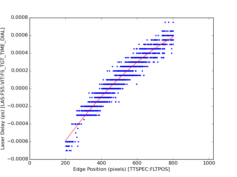
FIT RESULTS
fs_result = a + b*x + c*x^2,  x is edge position
------------------------------------------------
a = -0.001196897053
b = 0.000003302866
c = -0.

...

000000001349
------------------------------------------------
fit range (tt pixels): 200 <> 800
time range (fs):       -0.000590 <> 0.000582
------------------------------------------------

Unfortunately, right now CXI, XPP, and AMO have different methods for doing this calibration. Talk to your beamline scientist about how to do it and process the results.

Rolling Your Own

Hopefully you now understand how the timetool works, how the DAQ analysis works, and how to access and validate those results. If your DAQ results look unacceptable for some reason, you can try to re-process the timetool signal. If, right now, you are thinking "I need to do that!", you have a general idea of how to go about it. If you need further help, get in touch with the LCLS data analysis group. In general we'd be curious to hear about situations where the DAQ processing does not work and needs improvement.

There are currently two resources you can employ to get going:

1. It is possible to re-run the DAQ algorithm offline in psana, with e.g. different filter weights or other settings. This is documented extensively.
2. There is some experimental python code for use in situations where the etalon signal is very strong and screws up the analysis. It also simply re-implements a version of the DAQ analysis in python, rather than C++, which may be easier to customize. This is under active development and should be considered use-at-your-own-risk. Get in touch with TJ Lane <tjlane@slac.stanford.edu> if you think this would be useful for you.

...