...
Model | RA(°) | DEC(°) | Semi Major Axis (°) | Semi Minor Axis (°) | Pos.Ang.(°) |
283,990 | 1,355 | 0,300 | 0,190 | 327,000 | |
Pass 6 | 284.015(+/-0.004) | 1.392(+/-0.005) | 0.335(+0.117 -0.086) | 0.207 (+0.023 -0.021) | 330+/- 25 |
Pass 7 | 284.000(+/-0.006) | 1.374(+/-0.006) | 0.332(+0.109/-0.079) | 0.205 (+0.021/-0.017) | 327 +/-22 |
...
Fig. 8. Residual TSMap in which HESS J1857 is not fitted. Pass 6 analysis. + HESS contours

Fig 9. Residual TSMap in which HESS J1857 is not fitted. Pass 6 analysis. + HESS contours. Green crosses represents 2FGL sources.
Spectral analysis
We fitted the source using pointlike above 300GeV to prevent contamination at low energy.
We obtained the following SED and best fit using Pass 7 : 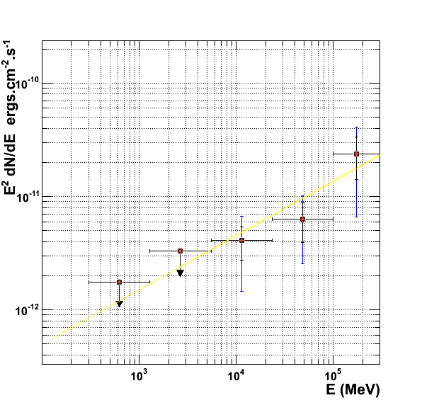
Fig. 10 : SED obtained using gtlike above 300 MeV. The best fit is show in yellow.
The source is fitted by a hard power law. The parameters of the best fit are those of the next table :
IRFS | Int. Flux (>100MeV) | -1 X Index | Lower limit (MeV) | Upper limit (GeV) | TS | gal |
|---|---|---|---|---|---|---|
Pass 7 | 5.67+/-0.65+/-3.2 | 1.65+/-0.27+/-0.31 | 100 | 100 | 28.1 | 1.09 |
Table. 5. Parameters of the best fit obtained using gtlike.
SED modeling
Section under construction
Adam constructed a time-dependent one-zone SED model with constant expansion velocity, and assuming a distance of 9 kpc. The modeling only need an IC component.

Fig. 11 show the SED modeling constructed by Adam. Blue point are those obtained with HESS data and the green one using ASCA observation. IC components : stellar (dot), IR (medium-dashed) and scattering on
CMB (long-dashed)
Preliminary fit:
Final B = 1.5 ± 1.0 ?G
Electron slope = 2.2 ± 0.1
Electron cutoff = 120 ± 40 TeV
Initial spin period = 13 ± 8 ms
Braking index = 2.5 ± 0.4
Theses parameters predict an age of 25 kyrs (21 kyrs predicted in Hessels et al. 2008 for the pulsar).
Discussion
Assuming a distance of 9kpc we derived the luminosity of the PWN to compute its gamma efficiency. We obtained :
L? (PWN) = 1.69 X 10^35 ergs/s.
Using the pulsar Edot =4.6 X 10^36 we computed an efficiency of 3.7%. To compare to the 3.1% obtained using HESS data.
This efficiency is consistent with what is expected from Ackerman et al. 2011 (the order of magnitude of the percent) as is shown in the following picture : 
Fig. 12 ?-ray Luminosity of the Pulsar Wind Nebulae as a function of the spin-down
luminosity of the associated pulsar. All the pulsar wind nebulae detected by Fermi are
associated with young and energetic pulsars. Pulsar wind nebulae detected by Fermi are
marked with red stars. Blue squares represent pulsars for which GeV ?-ray emission
seems to come from the neutron star magnetosphere, and not from the nebula.
In the paper
I'm now writting the draft of an A&A letter with M.-H. Grondin, M. Lemoine-Goumard, A.Van Etten, B. Stappers, A. Lyne, C. Espinoza.
The first part is an introduction of the source.
The second part summarize the data I used.
The third part is divided in
Bibliography :
(1) Abdo et al., Science, 327, 1103-1106, 2010