Data
From Siqi:
https://www.dropbox.com/s/8wrfbkpaosn23vq/labeledimg1.mat?dl=0
https://www.dropbox.com/s/uw9nx8mp8pqe94e/labeledimg2.mat?dl=0
In the data structure there is vccimg and yagimg which refer to the images on VCC and YAG screens. There is vccbox and yagbox which refer to the box coordinate where it finds the beam, [ystart yend xstart xend]. If it's empty it means it detects no signal. I corrected the mislabeled ones using the fitting method so they should all be labeled correctly now.
There is also a labedimg4.mat:
Some points worth mentioning:
1. the vccImg and yagImg are raw images, i.e. before background subtraction
2. background images are saved in vccbkg and yagbkg.
3. there is a camera gain problem on the VCC camera, so if you need to do background subtraction on VCC you may have to enforce non-negative intensities after subtraction. Background subtraction for YAG images work normally.
4. I also added in vccbeam and yagbeam which give the full beam image on both cameras. When I did the labeling I restrained the search region within the full beam region on these two images, since the vccImg and yagImg are just small portions of the full beam.
From David
I have downloaded the files, they are at (on the psana nodes) /reg/d/ana01/temp/davidsch/mlearn/acc_beam_locate/labeledimg*.mat
Access from Python
scipy can load mat files, here is some code that investigates a little:
In [3]: import scipy.io as sio
In [4]: labeledimg1 = sio.loadmat('labeledimg1.mat')
In [8]: vccImg = labeledimg1['vccImg']
In [18]: vccBox = labeledimg1['vccbox']
# you'll see vccImg and vccBox show up as 1 x 110 arrays of 'object', they are the images and labels for 110 samples

# like Siqi says, a box entry is empty if no beam is present, here we get a count of the non empty boxes, or samples with beam
In [23]: len([bx for bx in vccBox[0,:] if len(bx)>0])
Out[23]: 80

The first entry with a box is 4, so you can plot like
In [24] %pylab
In [26]: imshow(vccImg[0,4])
In [27]: bx = vccBox[0,4]
In [31]: ymin,ymax,xmin,xmax=bx[0,:]
In [32]: plot([xmin,xmin,xmax,xmax,xmin],[ymin,ymax,ymax,ymin,ymin], 'w')
In which case I see

Description
- Files 1 and 2 have 142 samples. With file 4, it is 239 samples.
- Each sample has a yag, vcc, and box for each - there are also backgrounds to subtract for file 4, and the beam to narrow the search.
- vcc values are in [0,255], and the boxed beam can get quite brite
- yag values go over 1000, I think, but the boxed value is always dim, like up to 14
First Pass - just files 1 and 2
We have to fit the 480 x 640 vcc images, and 1040 x 1392 yag images into 224 x 224 x 3 RBG images.
I thresholed yag at 255, then made grayscale images for each, using a scipy imresize option.
I generated codewords for the yag and vcc. The yag, which has bright beam, shows alot of structure:

These are plotted with a very large aspect ratio, the bottom is the 'nobeam' images.
However with the yag images, there is very little difference between nobeam and beam:
 There a
I suspect we will not be able to do much with these codewords without more preprocessing of the yag images - I think they are too faint for what vgg16 expects - it was trained on the imagenet color images.
Second pass
This problem seems harder than the localization for lasing fingers in amo86815. There is more variety in the signal we are trying to find. This leads to different kinds of signal processing pre-filtering of the images. Then sometimes the vgg16 codewords don't seem that homogenous - suggesting.
Of the 239 samples, 163 of the vcc have a labeled box. Below is a plot where we grab what is inside each box and plot it all in a grid - this is with the background subtraction for file 4. The plot on the left is before, and on the right, is after reducing the 480 x 640 vcc images to (224,224) for vgg16. We used scipy imreduce 'lanczos' to reduce (this calls PIL).

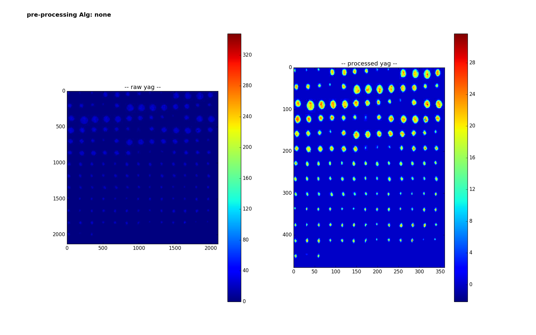
Here are the 159 smaples of the yag with a box - here are are using 'lanczos' to reduce from the much larger size of 1040 x 1392 to (224,224). It is interesting to note how the colorbar changes - the range no longer goes up to 320 - I think the 320 values were isolated pixels that get washed out? Or else there is something else I don't understand - we are doing nothing more than scipy.misc.imresize(img,(224,224), interp='lanczos',mode='F') but img is np.uint16 after careful background subtraction - (going through float32, thresholding at 0 before converting back)
Pipeline
Regression/box prediction
The processing pipeline for the regression
- choose a preprocessing algorithm
- create vgg16 codeword1 and 2 (8196 numbers, last two layers)
- separately for 'yag' and nm'
- for each of the for each of the 163 (or 159) samples,
- train a linear regression classifier on the remaining 162 (or 158) samples
- map from 8196 variables to 4
- use it to predict a box for the ommitted sample
- optionally - limit input features - reject features with variance less than threshold
- (maybe they are noisy and throwing off classifier)
- train a linear regression classifier on the remaining 162 (or 158) samples
- for each of the for each of the 163 (or 159) samples,
Measure accuracy
For localization - on a shot by shot basis, where we are comparing boxA to boxB, one typically calculated the ratio of area of the intersection to area of the union. For imagenet competitions, one gets success on a shot/image of inter/union >=0.5, those predictions look quite good! One can then come up with a overall accuracy based on the inter/union threshold. Below, we report on accuracy for different thresholds, .5, .2 and .01 - the latter is to see how accurate we are at getting any overlap.
To visualze the results, we make a similar plot to above, but plot the truth box in white, and the predicted box in red.
Results
Pre processing=None, files=1,2,4
For the vcc, accuracies, a 1% overlap is 55%

For the yag, a 1% overlap is 86%:

All Accuracies
36 different runs were carried out, varying each of the following:
- Pre-processing algorithm, one of
- none
- just 'lanczos' reduction
- denoise-log
- 3 pt median filter
- log(1+img)
- 'lanczoz' reduction
- multiply by scale factor
- denoise-max-log
- 3 pt median filter
- 3 x 3 sum
- 3 pt median filter
- 'max_reduce' (save largest pixel value over square)
- 'lanczoz' reduction (to get final (224,224) size)
- log(1+img)
- scale up
- none
- files, one of
- just 1,2
- 1,2,4
- Do and Don't subtract background for file 4
- Do and Don't filter out some of the 8192 features with variance <= 0.01 before doing regression
Below is a table of all these results
Best Result - YAG
The best 1% overlap for the YAG is 92%
- It is over files 1,2,4
- used denoise-log, and subtracts the background.
- Same result with/without the variance feature selection
- Not subtracting the background reduced the accuracy to 89%.
- Not using file 4 reduced accuracy to 90%.
- Using the denoise-max-log led to 84% accuracy (worse than no preprocessing = 86%).

Best Result - VCC
The best 1% overlap for the VCC is 76%.
- It is over files 1,2
- used denoise-log
- adding file 4, with subbkg, reduced acc to 63%
- adding file 4, without subbkg reduced acc to 48%
