Introduction
Omega3P is a parallel finite-element electrogmagnetic code for high-fidelity modeling of cavities. It calculates the resonant frequencies and other rf parameters of a cavity, as well as damping effects due to external couplings. It uses Nedelec-type hierarchical vector basis up to 6th order with quadratic (10-points) tetrahedral elements for improved solution accuracy.
Mathematical Modeling
Lossless cavities
Maxwell's equations in the frequency domain for a perfectly conducting cavity can be written as the following PDE,
\begin
\nabla \times \left(\frac
\nabla \times \vec
\right) - k^2 \epsilon \vec
& = 0 & on \quad \Omega
\vec
\times \vec
& = 0 & on \quad \Gamma_
\vec
\times \left( \frac
\nabla \times \vec
\right) & = 0 & on \quad \Gamma_
\end
We use Neelec-type vector basis functions to discretize the electric field:
[\vec
=\sum_i x_i \vec
_i]
We obtain the following generalized eigenvalue problem:
\begin
= k^2
\quad where &
_
= \int_
\left( \nabla \times \vec
_i \right) \cdot \frac
\left( \nabla \times \vec
_j \right) d\Omega &
_
= \int_
\vec
_i \cdot \epsilon \vec
_j d\Omega &
\end
The matrix K is real symmetric while M is real symmetric positive definite. If there are lossy materials in the cavity, the matrix M and/or K will be complex.
Waveguide loaded cavities
For modeling waveguide-loaded cavities, we use either the absorbing boundary condition (ABC) or the waveguide boundary condition (WBC). The following picture illustrates a cavity with 3 waveguides, and each of them is modeled with ABC.
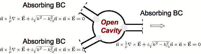
The discretized system is a complex nonlinear eigenvalue problem,
[
+ i \sum_j \sqrt{k^2-k^2_{cj}}
_j
= k^2
]
where the damping matrix W is
[
(
j)
= \int_
\left( \vec
\times \vec
_m \right) \cdot \left( \vec
\times \vec
_n \right) d\Gamma
]
The following picture illustrates a cavity with waveguides, which are modeled with WBC.
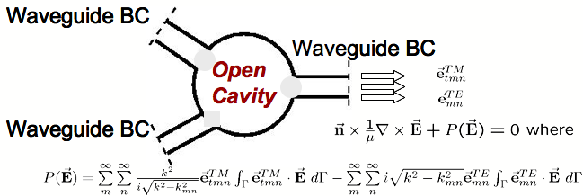
The corresponding discretized system becomes a complex nonlienar eigenvalue problem,
[
+ i \sum_
\sqrt{k^2-(k^
_
)^2}
^
_
+ i \sum_
\frac
{\sqrt{k^2-(k^
_
)^2}}
^
TM _
= k^2
]
where the waveguide matrices are
[
(
^
_
)_
= \int_
\vec
^
_
\cdot \vec
i d\Gamma \int
\vec
^
_
\cdot \vec
_j d\Gamma
]
[
(
^
_
)_
= \int_
\vec
^
TM _\cdot \vec
i d\Gamma \int
\vec
^TM _
\cdot \vec
_j d\Gamma
]
Numerical Methods
The following is a graphical description of the four different types of physics problems that Omega3P can solve and the solver options that can be used.