Decision Theoretic Approach

Overview

In this project we study and investigate network anomaly detection algorithms [1], [2] and [3] for Internet Paths. We also develop a Decision Theoretic Approach (DTA) based on our observations regarding the characteristics of the performance-measurement statistics obtained from the IEPM-BW project.

To study and compare the algorithms we use the data sets collected by IEPM-BW spanning approximately 2 years (i.e. 2006 - 2008). The Internet paths observed were the links between Stanford Linear Accelerator Center (SLAC) and the following sites:

1. San Diego Supercomputing Center (SDSC) USA,
2. Oak Ridge National Laboratory (ORNL) USA,
3. European Organization for Nuclear Research (CERN) Geneva, Switzerland,
4. Forschungszentrum Karlsruhe (FZK) Germany,
5. Deutsches Elektronen-Synchrotron (DESY) Germany,
6. University of Toronto (UTORONTO) Canada and
7. National Laboratory for Particle and Nuclear Physics (TRIUMF) Canada.

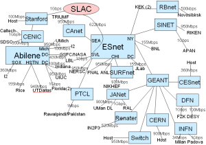
The topology of the monitoring framework is shown in figure 1.

Data Sets

The data sets used in the study may be downloaded from the links listed below. These data sets were collected by the IEPM-BW project and the latest performance statistics may be accessed from here.

Table 1: Performance measurement statistics compiled by IEPM, as seen from SLAC.

Download the complete data archive [zip 10 MB] or [7z 8 MB]

Labeling and Detection Algorithms

To perform a fair comparison between [1], [2], [3] and the proposed DTA we devised a labeling algorithm to identify true anomalies in the data sets. This labeled data was then used to determine the accuracy (true-positive rate), corresponding false-positive rate and the detection delay. The labeling algorithm and the decision theoretic approach for real-time anomaly detection are discussed at length in the research paper. (The paper will be posted soon.)

Implementations and Parameter Tuning

The source code of the implementations and the tuning of parameters is discussed below. Please consider two important factors while we discuss the parameters tuning: a) We define an anomalous event as one which significantly varies from the normal behaviour of the Internet Path and the perturbation persists for at least three hours. b) The measurements made by IEPM-BW are at least 45 mins apart.

a) Plateau Algorithm

The Plateau Algorithm [1] takes four input parameters - history buffer length, trigger buffer length, sensitivity and threshold. We define the trigger buffer length to hold observations spanning at least 3 hours (since we define an anomalous event as one that persists for at least 3 hours). Since the measurements made by IEPM are 45 mins apart, we get about 6 observations. We then empirically determine the optimal length of the history buffer to span at least 5 days ~ 240 observations.

We initially define the sensitivity as one (1) and determine the optimal threshold value for each link (i.e. the value with the optimal ratio of true-positives to false positives). As suggested by the authors, this threshold falls between 30%-40%. Finally for the history buffer length, the trigger buffer length and the optimal threshold, we vary the sensitivity to determine the spectrum of the ratio of true-positive rate to false positive rate. Based on the observations we plot the ROC curves as shown in figure 2. One set of data points is shown in table 2.

Table 2: Results compiled by Plateau algorithm when analyzing the Internet path between SLAC and DESY.

Legend:
H - History buffer length, TB - Trigger buffer length, TH - threshold, S - sensitivity, TP - true positives obtained, FP - false positives obtained, #P - true positives, N~days - days observed, TPR - true positive rate, FPR - false positive rate.

The source code of the implementation is available in C# [cs] and perl [pl]

b) Adaptive Fault Detection

The Adaptive Fault Detection [3] method employs four parameters - the desidred detection rate, the desired false positive rate, the history buffer length and the observed window length. We use the values as suggested by the author and for observed window length of 20, a history buffer length of 100 and the desired detection rate of 0.95 and we vary the desired false positive rate to obtain the spectrum of the ratio of true-positive rate to false positive rate. Based on the observations we plot the ROC curves as shown in figure 2. One set of data points is shown in table 3.

Table 3: Results compiled by Adaptive Fault Detection (ADF) method when analyzing the Internet path between SLAC and DESY.

Legend:
HN - History buffer length, a - desired false positive rate, B - desired detection rate, N - observed window length, TP - true positives obtained, FP - false positives obtained, #P - true positives, N~days - days observed, TPR - true positive rate, FPR - false positive rate.

The source code of the implementation is available in C# [cs].

c) Kalman Filters

The Kalman Filter [2] method employs two input parameters - the observed window length and the Kalman gain. We use the values as suggested by the author and for the observed window length and vary the kalman gain to obtain the spectrum of the ratio of true-positive rate to false positive rate. Based on the observations we plot the ROC curves as shown in figure 2. One set of data points is shown in table 4.

Table 4: Results compiled by Kalman Filters (KF) method when analyzing the Internet path between SLAC and DESY.

Legend:
W- observed window length, K - kalman gain, TP - true positives obtained, FP - false positives obtained, #P - true positives, N~days - days observed, TPR - true positive rate, FPR - false positive rate.

The source code of the implementation is available in C# [cs]. (not up to date, will be revised soon)

d) Decision Theoretic Approach

Decision Theoretic Approach employs four parameters - the desired false positive rate (alpha), the desired detection rate (beta), the history buffer length and the low-pass median filter length. We apply the median filter of length 7 to remove the high frequency component. We then determine the optimum history buffer length by empirical observation. This turns out to be 90. Opting for the maximum detection rate of 0.99, we vary the desired false positive rate to obtain the entire spectrum of the ratio of true-positive rate to false positive rate. Based on the observations we plot the ROC curves as shown in figure 2. One set of data points is shown in table 5.

This algorithm use three parameters one is threshold which is calculated in terms of Alpha and Beta, and other two are buffer lengths (History buffer and n-Tap Median filter). Same scheme is used for this algorithm, such that minimum value of n = 7 is used for n-Tap Median filter with some appropriate value of History buffer. By keeping these values same and changing different values of Alpha and Beta (Threshold) for each dataset ROCs are generated.

Table 5: Results compiled by the proposed DTA when analyzing the Internet path between SLAC and DESY.

Legend:
H - History buffer length, a - desired false positive rate, B - desired detection rate, n-tap - median filter length, TP - true positives obtained, FP - false positives obtained, #P - true positives, N~days - days observed, TPR - true positive rate, FPR - false positive rate.

The source code of the implementation is available in C# [cs] and perl [pl] (utilityFunctions [pm], conf).

References

1. C. Logg, L. Cottrell, and J. Navratil. Experiences in traceroute and available bandwidth change analysis. In NetT '04: Proceedings of the ACM SIGCOMM workshop on Network troubleshooting, pages 247-252. ACM, 2004.
2. A. Soule, K. Salamatian, and N. Taft. Combining filtering and statistical methods for anomaly detection. In Internet Measurement Conference (IMC 2005), pages 331-344. USENIX, 2005.
3. H. Hajji. Statistical analysis of network traffic for adaptive faults detection. In IEEE Transactions on Neural Networks, pages 1053-1063, 2005.