Introduction

If you want a quick start, a 17-line example script you can run is Here.

We also highly recommend learning by running the small examples Here.

This document offers an overview of the psana analysis framework for user scripts written in the Python programming language. It allows its users to benefit from a rich set of services of the core framework while retaining full control over an iteration in data sets (runs, files, etc.). This combination makes it possible for the interactive exploration and (if needed) visualization of the experimental data. Note that by the latter we always mean data files in the XTC or HDF5 formats produced by the LCLS DAQ or Data Management system. We also suggest visiting the Glossary of Terms which is found in the end of the document.

The following usage scenario represents the core "philosophy" of the interface:

1. in order to access a data (from a single file, or a collection of files belonging to a run, or files of multiple runs) a user has to write a Python script. There are no restrictions on how the script is written, or which other Python modules are used by the script.
2. in that script the user imports a special module called psana. The module provides an interface to the services of the core framework. The psana module is no different than any other modules imported into the script.
3. the user opens a data set using a special function (provided by the module) similarly to opening regular files
4. at this point the experimental data (so called events) can be read in a way which is conceptually similar to how data records are read from a regular file
5. each such event obtained from the data set is a complex object whose content can be explored by calling various methods returning components of the events as well as various meta-information
6. in addition to events the framework also allows access to the event environment information, which incorporates things like EPICS variables, etc.

The rest of the document will map that "philosophy" into practical steps which would need to be taken along that path. We will also cover the basic principles of the psana API as well as their behavioral aspects. Keep in mind that the implementation of the psana python scripts is based on its core psana. Hence there are many commonalities which are shared by these tools, including:

• the transient Event Model
• the transient Environment Model
• naming convention for detector components
• a collection of Python classes representing detector components
• the job configuration service and the syntax of the configuration files
• modules written for the batch version of psana

A reader of the document isn't required to be fully familiar with the batch framework. Those areas where such knowledge would be needed are expected to be covered by the document. Though, we still encourage our users to spend some time to get an overview of the Data Analysis Tools we provide at PCDS. That's because many problems in doing the data analysis can be solved by the batch version of psana in a more efficient and natural way. These two flavors of the framework are not meant to compete with each other, they are designed to complement each other to cover a broader spectrum of analysis scenarios.

Setting up the analysis environment

There are three steps which need to be performed in order to get access to this API and the data for your experiment:

1. obtain and properly configure your UNIX account at PCDS. Specific instructions can be found in the Account Setup section of the Analysis Workbook.

2. ssh to a psana machine. Do not do analysis on pslogin or psexport. After ssh-ing to pslogin, continue to the psana system.

The later command should be done just once per session. It will initialize all relevant environment variables, including PATH, LD_LIBRARY_PATH, PYTHONPATH and some others. This will also give you an access to an appropriate version of the Python interpreter and the corresponding Python modules. We recommend using ipython. The following example illustrates how to launch the interpreter and test if the psana python module is available in the session environment. When everything is set up correctly one should see:

% ipython

Python 2.7.2 (default, Jan 14 2013, 21:09:22)
Type "copyright", "credits" or "license" for more information.

IPython 0.13.1 -- An enhanced Interactive Python.
?         -> Introduction and overview of IPython's features.
%quickref -> Quick reference.
help      -> Python's own help system.
object?   -> Details about 'object', use 'object??' for extra details.

In [1]: import psana

In [2]: psana.
Display all 108 possibilities? (y or n)
psana.Acqiris            psana.Gsc16ai            psana.ndarray_float32_1  psana.ndarray_int32_5    psana.ndarray_uint32_3
psana.Andor              psana.Imp                psana.ndarray_float32_2  psana.ndarray_int32_6    psana.ndarray_uint32_4
psana.Bld                psana.Ipimb              psana.ndarray_float32_3  psana.ndarray_int64_1    psana.ndarray_uint32_5
psana.BldInfo            psana.Lusi               psana.ndarray_float32_4  psana.ndarray_int64_2    psana.ndarray_uint32_6
..

The first application

Here is the psana version of the traditional "Hello World!" program:

from psana import *

dataset_name = "exp=CXI/cxitut13:run=22"
ds = DataSource(dataset_name)

for num,evt in enumerate(ds.events()):
    id = evt.get(EventId)
    print "Event #",num," has id:",id

The code of this example does nothing but scanning through all events of the data set and reporting identifiers (class EventId) of each event (class Event). The identifiers () encapsulate a number of attributes, including: timestamp, fiducials, etc. And here is how the output should look like:

Event # 0  has id: XtcEventId(run=22, time=2013-01-18 17:58:53.047288760-08, fiducials=19404, ticks=331022, vector=1)
Event # 1  has id: XtcEventId(run=22, time=2013-01-18 17:58:53.055622526-08, fiducials=19407, ticks=330630, vector=2)
Event # 2  has id: XtcEventId(run=22, time=2013-01-18 17:58:53.063956294-08, fiducials=19410, ticks=329468, vector=3)
..

Now let's go through the example's code line-by-line and see what it does at each step:

1. importing all definitions from the psana module into the global namespace. This includes functions, classes and types:

   from psana import *
   

2. opening a data set and checking if it exists/available to your process:

   dataset_name = "exp=CXI/cxitut13:run=22"
   ds = DataSource(dataset_name)
   

3. iterating over all events in the data set and obtaining an event identification object for each event:

   for num,evt in enumerate(ds.events()):
       id = evt.get(EventId)
   

Please, note that the following definitions mentioned in the example were imported from the psana module:

• DataSource is a function for locating and opening data sets
• Event is a type (class) representing transient (in-memory) event objects.
• EventId is a type (class) which is used as a primary key to fetch the event identity object from an event.

More details on parameters of the get() function will be provided later in this document. The module exports many other definitions. Some of them will be introduced and explained in the rest of the document as needed.

Data set specification

The data set string encodes various parameters, some of which are needed to locate data files, while others would affect the behavior of the file reader. The general syntax of the string is:

par[=val][:par[=val][...]

These are some of the parameters which are supported in psana:

• experiment name (which may optionally contain the name of an instrument)

  exp=cxi12313
  exp=CXI/cxi12313
  

• run number specification (can be a single run, a range of runs, a series of runs, or a combination of all above):

  run=1
  run=10-20
  run=1,2,3,4
  run=1,20-20,31,41
  

• file type (presently the default type is 'xtc')

  xtc
  h5
  

• a set of streams belonging to dataset which is a comma-separated list of stream ranges, range can be a single stream number or two number separated by dash:

  stream=0,2-4,11
  stream=2
  

• allow reading from live files while they're still being recorded (by the DAQ or by the Data Migration service). Note that this feature is only available when running psana at PCDS nodes, in all other cases the option will be ignored:

  live

• a non-default directory where xtc files are located:

  dir=/reg/d/ffb/xpp/xpptut15/xtc

Putting all together one would see a data set specification which would tell the framework to read data of stream #2 from XTC files of run 41 while these files were sill being recorded (by the DAQ, or the data migration service, or by another process of the same user, etc.):

exp=CXI/cxi12313:run=41:xtc:stream=2:live

The complete description of the data set string syntax and allowed parameters can be found in the specification document.

Extracting data from an event

Detector Names

In a given event, one can get a list of all detector names (and aliases) to use in the examples below with a script similar to the following:

from psana import *
ds = DataSource('exp=cxi86715:run=99')
for evt in ds.events():
    print evt.keys()
	break # to stop the loop over events

Simple Area-Detector Data Access

There is a simple "one-line" python interface to access area-detector information (e.g. cspad, epix, pnccd etc.) including dark corrections, bad-pixel suppression, common-mode correction and application of detector metrology:

from psana import *
ds  = DataSource('exp=cxi86715:run=99')
src = Source('DsaCsPad')
det = Detector(src, ds.env())
for evt in ds.events():
    print det.image(evt) # returns a 2D corrected image using deployed metrology

Note that the image() method does not currently do other corrections, e.g. per-pixel-gain, but other correction values (like per-pixel-gain) can be retrieved with a similar one-line call, and then multiplied in one-line of python.

There is a lot of other information accessible through the Detector class (e.g. pixel locations, calibration constants, various masks).  For a more complete list, see /reg/g/psdm/sw/releases/ana-current/Detector/examples/ex_all_dets.py.  We are working on expanding this interface to work for all detector types.

More General Data Access

In this section we're going to focus on an event object to see how to get various information from it. Let's begin with an example where we're fetching and plotting an image captured at the Princeton camera (which is one of the detectors available at the XCS instrument). In this example we won't be iterating over all events. Only the first event will be considered:

from psana import *

ds = DataSource('exp=XCS/xcstut13:run=15')
src = Source('DetInfo(XcsBeamline.0:Princeton.0)')

itr = ds.events()
evt = itr.next()
frame = evt.get(Princeton.FrameV1, src)

import matplotlib.pyplot as plt

plt.figure('Princeton Camera')
plt.imshow(frame.data())
plt.show()

This code introduces two new things which weren't present in the "Hello World" code:

• the get() method is called with two parameters:
  1. the expected type of an event component
  2. the expected address (source) of a component within an event
• Princeton.FrameV1 which is a type of the Princeton camera object returned by the get() method

Four forms of the get() method

The psana event contains objects which may have different origins, such as:

• the LCLS DAQ system
• external psana modules (for example the calibrations or frame reconstruction modules)
• the psana framework itself (such as the event identifier)
• the user's psana python script (the code can use the event's put() method to extend the event before passing it to another algorithm in the workflow/processing pipeline within the same Python application)

Things are getting further complicated by the following factors:

• the DAQ system may produce more than one object for a particular detector, each of which would needed to be unambiguously identified in the event container
• the external psana modules or the Python script may add more versions for the same detector object as a result of data processing (calibration, etc.)

In order to deal with all these object addressing requirements psana introduces three keys which allows to uniquely identify a particular object within the event:

• type - is the primary (mandatory) parameter specifying an expected type of an object within the framework
• src - is some sort of an address of a component within an event. The address parameter is not required for some types of components. Actually, the very first ("Hello World!") example of this Introduction just illustrated it. Technically, the source information is encapsulated into a special object which is produced by the constructor of class Source.
• key - is an optional string which is mainly meant to be used to name various stages of processing for the same kind of a detector (though, it's not really limited to a specific detector).

The combination of these keys led to the following collection of signatures supported by the method:

• get(type, src, key) - the full form of the method
• get(type, src) - the shortcut form of the method which is equivalent to get(type, src, "")
• get(type, key) - is another shortcut which is similar to get(type, Source(None), key)
• get(type) - is the shortest form which is equivalent to get(type, Source(None), "")

The type key is a real Python type known to the framework. All types which would be recognized by a particular version of the framework can be obtained by the 'dot' operator of the ipython interpreter as shown below:

% ipython

In [1]: import psana

In [2]: psana.
Display all 108 possibilities? (y or n)
psana.Acqiris            psana.Gsc16ai            psana.ndarray_float32_1  psana.ndarray_int32_5    psana.ndarray_uint32_3
psana.Andor              psana.Imp                psana.ndarray_float32_2  psana.ndarray_int32_6    psana.ndarray_uint32_4
psana.Bld                psana.Ipimb              psana.ndarray_float32_3  psana.ndarray_int64_1    psana.ndarray_uint32_5
psana.BldInfo            psana.Lusi               psana.ndarray_float32_4  psana.ndarray_int64_2    psana.ndarray_uint32_6
psana.Camera             psana.OceanOptics        psana.ndarray_float32_5  psana.ndarray_int64_3    psana.ndarray_uint64_1
psana.ControlData        psana.Opal1k             psana.ndarray_float32_6  psana.ndarray_int64_4    psana.ndarray_uint64_2
psana.CsPad              psana.Orca               psana.ndarray_float64_1  psana.ndarray_int64_5    psana.ndarray_uint64_3
psana.CsPad2x2           psana.PNCCD              psana.ndarray_float64_2  psana.ndarray_int64_6    psana.ndarray_uint64_4
psana.DataSource         psana.PSAna              psana.ndarray_float64_3  psana.ndarray_int8_1     psana.ndarray_uint64_5
..

Note that some of those entries aren't really types. Besides, they may be nested Python modules providing more types like this one:

In [3]: psana.Princeton.
psana.Princeton.Config    psana.Princeton.ConfigV3  psana.Princeton.Frame     psana.Princeton.Info
psana.Princeton.ConfigV1  psana.Princeton.ConfigV4  psana.Princeton.FrameV1   psana.Princeton.InfoV1
psana.Princeton.ConfigV2  psana.Princeton.ConfigV5  psana.Princeton.FrameV2

The second (source) key should be constructed using a special class called Source which also exported by the psana module:

src = Source('<object address string>')

The format of the object address string varies between different kinds of objects, and in general it's related to an origin of a desired object.

And the last key is an optional string which is called key. Its primary use is to disambiguate between different versions of the same kind of information within the event. In the current practice raw data which originate from the DAQ system would always have this key empty. If there is an external psana module processing that raw data and turning it in some more convenient to use form (calibrated, reconstructed, reduced, restructured, etc.) then that second version would get some non-trivial key value, like: "v1", "processed", "calibrated", etc. A specific name of the key is solely under a discretion of the corresponding module (user's code). The combinations of types, sources and keys allows users to build very powerful workflows on top of psana.

The ipython interpreter makes it easy to explore the namespace of the framework module to see what's available. This unfortunately doesn't address the question - "Now, as I have my event, how do I know what's in that event, which form of the get() method should I use, and which specific values of parameters should I put? Unless you already know the answer, proceed to the next section to find the one!

Browsing through a catalog of objects stored within an event

The following example demonstrates how to dump a catalog of event components:

In [8]: evt.keys()
Out[8]:
[EventKey(type=psana.EvrData.DataV3, src='DetInfo(NoDetector.0:Evr.0)'),
 EventKey(type=psana.Camera.FrameV1, src='DetInfo(CxiDg1.0:Tm6740.0)'),
 EventKey(type=psana.Camera.FrameV1, src='DetInfo(CxiDg2.0:Tm6740.0)'),
 EventKey(type=psana.CsPad.DataV1, src='DetInfo(CxiDs1.0:Cspad.0)'),
 EventKey(type=psana.Bld.BldDataEBeamV3, src='BldInfo(EBeam)'),
 EventKey(type=psana.Bld.BldDataFEEGasDetEnergy, src='BldInfo(FEEGasDetEnergy)'),
 EventKey(type=psana.EventId),
 EventKey(type=None)]

In [9]:

The information reported by the method would give us an idea what's found in the event, and how to obtain those components using the get() method. When psana has been imported into the global namespace, the mapping is:

from psana import *
...
obj1 = evt.get( EvrData.DataV3,             Source('DetInfo(NoDetector.0:Evr.0)'))
obj2 = evt.get( Camera.FrameV1,             Source('DetInfo(CxiDg1.0:Tm6740.0)'))
obj3 = evt.get( Camera.FrameV1,             Source('DetInfo(CxiDg2.0:Tm6740.0)'))
obj4 = evt.get( CsPad.DataV1,               Source('DetInfo(CxiDs1.0:Cspad.0)'))
obj5 = evt.get( Bld.BldDataEBeamV3,         Source('BldInfo(EBeam)'))
obj6 = evt.get( Bld.BldDataFEEGasDetEnergy, Source('BldInfo(FEEGasDetEnergy)'))
obj7 = evt.get( EventId)

Few notes on that output:

• the last component (the one which has type=None) reported by the keys() method should be ignored. This is an artifact of the current implementation of this API. It may go away in some future release of the software. We mention it here just to address possible confusion which users may have when seeing this output.
• note the variations in the syntax of the components' addresses.

Working with a list of keys

For those would like to build some automation in discovering which components and of what kind exist in the event there is another option. A user can iterate over the list of key elements to examine their attributes. Each such element would encapsulate a type, a source and a key (string) of the corresponding event component. Consider the following example:

for k in evt.keys():
    print "type:   ", k.type()
    print "source: ", k.src()
    print "key:    ", k.key()
    ..

The type() method will return one of those Python type objects which were already mentioned in section "Four forms of the get() method". If a user is looking for a key which has a specific type then the following type comparison can be used:

for k in evt.keys():
    if k.type() == Camera.FrameV1:
        print "got Camera.FrameV1"

The src() method would return an object of class Src which is an abstraction (base class) for specific classes of data sources. At the time when this document was being written, there were three kinds of sources:

• detector-level addresses (class DetInfo)
• addresses for BLD devices (class BldInfo)
• event processing information (class ProcInfo)

Since APIs of those specific source classes differ one from another then a user would need to obtain the final type using the following technique:

for k in evt.keys():
    src = k.src()
    src_type = type(src)
    if   src_type == DetInfo  : print "detector name: ", src.detName(), " device name:   ", src.devName(), ...
    elif src_type == BldInfo  : print "detector type: ", src.type(),    " detector name: ", src.detName(), ...
    elif src_type == ProcInfo : print "IP address:    ", src.ipAddr(),  " process id:    ", src.processId()

Look for the documentation of the source classes to get a full description of the classes' methods.

Finally, the last method key() returns a string representing an optional third key which was already explained in section "Four forms of the get() method". In most cases the method will return an empty string.

Other operations with events

The event object also provides two operations for manipulating the contents of the event: adding more or removing existing components. Signatures of both operations are very similar to the ones of method get(). Specifically these are four forms of method remove():

• remove(type, src, key) - the full form of the method
• remove(type, src) - the shortcut form of the method which is equivalent to remove(type, src, "")
• remove(type, key) - is another shortcut which is similar to remove(type, Source(None), key)
• remove(type) - is the shortest form which is equivalent to remove(type, Source(None), "")

And similar forms for method put():

• put(obj, type, src, key) - the full form of the method
• put(obj, type, src) - the shortcut form of the method which is equivalent to put(obj, type, src, "")
• put(obj, type, key) - is another shortcut which is similar to put(obj, type, Source(None), key)
• put(obj, type) - is the shortest form which is equivalent to put(obj, type, Source(None), "")

Note that method put() has an additional parameter for a new object which is expected to be added to the event.

And the last method of the event API will return a run number. This information may be useful for data sets spanning across many runs:

ds = DataSource("exp=CXI/cxitut13:run=22,23,24,25)
for evt in ds.events():
    print "run: ", evt.run()
    ..

Accessing event environment data

The event environment encapsulate a broad spectrum of data and services which have various origins. This environment is needed to evaluate or process event data in a proper context. Some of these data may have different life cycles than events. Other parts of this information (such as calibrations) may not even come directly from the input data stream (the DAQ system). The information is available through a special object which is obtained by calling the data set object's method env():

dsname = 'exp=MEC/mec70813:run=35'
ds = DataSource(dsname)

env = ds.env()
env.
env.calibDir     env.configStore  env.expNum       env.fwkName      env.hmgr         env.jobName
env.calibStore   env.epicsStore   env.experiment   env.getConfig    env.instrument   env.subprocess

The same environment object can also be obtained by calling a similar method of classes Run.env() and Step.env(). The environment can be split into a number of categories which are explained in a dedicated sub-subsection below.

Job configuration information

Methods found in this category are meant to be used for information purposes. Though, one of their practical uses could be to create output (log, data, etc.) files which would have unique yet meaningful names relevant to an input data set and a job processing the data:

• expNum(): a numeric identifier of the corresponding experiment
• experiment(): the name of the experiment
• jobName(): the unique name of the job (this may be used by the users code to create output log files which would have unique yet meaningful names)
• subprocess(): the process number in a multi-process version of the framework (at the moment the method will always return 0. See details at section "MPI Parallelization")
• instrument(): the name of the instrument

This is a sample analysis session illustrating a result of calling the methods:

ds  = DataSource('exp=CXI/cxitut13:run=22')
env = ds.env()

print '   framework name:',env.fwkName()
print '         job name:',env.jobName()
print '       instrument:',env.instrument()
print '    experiment id:',env.expNum()
print '  experiment name:',env.experiment()
print 'subprocess number:',env.subprocess()

This will produce an an output which will look like this:

   framework name: psana
         job name: cxitut13:run=22
       instrument: CXI
    experiment id: 304
  experiment name: cxitut13
subprocess number: 0

Calibration Store

There are two methods in this category:

• calibDir(): the path name to a directory with calibration constants
• calibStore(): the interface to a repository of the calibration constants

The second method would return an object of the generic environment container class EnvObjectStore . Specific details of this interface are beyond a scope of the present document. The Calibration Store is mainly used by special calibration modules.

Configuration Store

This Store encapsulate various detector/device configuration information which is typically (in reality - it may vary) recorded by the DAQ system at the beginning of each run.

Consider the following example in which the first try to list configuration keys will result in an empty dictionary:

ds = DataSource('exp=CXI/cxitut13:run=22')
configStore = ds.env().configStore()
configStore.keys()

[]

The second attempt made after getting to the first event will produce some meaningful output:

itr = ds.events()
evt = itr.next()
configStore.keys()

[EventKey(type=psana.ControlData.ConfigV2, src='ProcInfo(0.0.0.0, pid=17877)'),
 EventKey(type=None, src='ProcInfo(0.0.0.0, pid=17877)'),
 EventKey(type=psana.EvrData.ConfigV7, src='DetInfo(NoDetector.0:Evr.0)'),
 EventKey(type=None, src='DetInfo(NoDetector.0:Evr.0)'),
 EventKey(type=psana.EvrData.ConfigV7, src='DetInfo(NoDetector.0:Evr.1)'),
 EventKey(type=None, src='DetInfo(NoDetector.0:Evr.1)'),
 EventKey(type=psana.EvrData.ConfigV7, src='DetInfo(NoDetector.0:Evr.2)'),
 EventKey(type=None, src='DetInfo(NoDetector.0:Evr.2)'),
 EventKey(type=psana.Epics.ConfigV1, src='DetInfo(EpicsArch.0:NoDevice.0)'),
 EventKey(type=None, src='DetInfo(EpicsArch.0:NoDevice.0)'),
 EventKey(type=psana.Epics.ConfigV1, src='DetInfo(EpicsArch.0:NoDevice.1)'),
 EventKey(type=None, src='DetInfo(EpicsArch.0:NoDevice.1)'),
 EventKey(type=psana.Acqiris.ConfigV1, src='DetInfo(CxiEndstation.0:Acqiris.0)'),
 EventKey(type=None, src='DetInfo(CxiEndstation.0:Acqiris.0)'),
 EventKey(type=psana.Ipimb.ConfigV2, src='DetInfo(CxiEndstation.0:Ipimb.0)'),
 EventKey(type=psana.Lusi.IpmFexConfigV2, src='DetInfo(CxiEndstation.0:Ipimb.0)'),
 EventKey(type=None, src='DetInfo(CxiEndstation.0:Ipimb.0)'),
 EventKey(type=None, src='DetInfo(CxiEndstation.0:Ipimb.0)'),
 EventKey(type=psana.Camera.FrameFexConfigV1, src='DetInfo(CxiEndstation.0:Opal4000.1)'),
 EventKey(type=psana.Opal1k.ConfigV1, src='DetInfo(CxiEndstation.0:Opal4000.1)'),
 EventKey(type=None, src='DetInfo(CxiEndstation.0:Opal4000.1)'),
 EventKey(type=None, src='DetInfo(CxiEndstation.0:Opal4000.1)'),
 EventKey(type=psana.Ipimb.ConfigV2, src='DetInfo(CxiDg1.0:Ipimb.0)'),
 EventKey(type=psana.Lusi.IpmFexConfigV2, src='DetInfo(CxiDg1.0:Ipimb.0)'),
 ..

The configuration keys have a structure which is reminiscent to the one of the event keys. This is illustrated below:

In [140]: configStore.
configStore.get   configStore.keys

In [142]: keys = configStore.keys()

In [143]: keys[4]
Out[143]: EventKey(type=psana.EvrData.ConfigV7, src='DetInfo(NoDetector.0:Evr.1)')

In [144]: keys[4].type()
Out[144]: psana.EvrData.ConfigV7


In [145]: obj = configStore.get(EvrData.ConfigV7,Source('DetInfo(NoDetector.0:Evr.1)'))

In [146]: obj.
obj.eventcodes   obj.neventcodes  obj.noutputs     obj.npulses      obj.output_maps  obj.pulses       obj.seq_config

In [147]: type(obj)
Out[147]: psana.EvrData.ConfigV7

The get() method of the Configuration Store will return objects describing the corresponding components of the events. The configuration objects are explained in "The psana Reference Manual". As an example, here is a direct link to the documentation of class EvrData.ConfigV7.

ControlPV

ControlPV is a configuration data which is updated on every step (steps are explained later in the document when discussing various ways of iterating over events in a data set). Like any other configuration data it is accessible through the environment object. Here is an example of getting controlPV data:

from psana import *

ds = DataSource('exp=xpp66613:run=300:h5')

for step in ds.steps():
    control = ds.env().configStore().get(ControlData.Config)
    print [(c.name(), c.value()) for c in control.pvControls()]

This will result in the following output:

[('lxt_ttc', -1.9981747581849466e-12)]
[('lxt_ttc', -1.8004943676675365e-12)]
[('lxt_ttc', -1.6001426205245978e-12)]
[('lxt_ttc', -1.3997908733800049e-12)]
[('lxt_ttc', -1.199439126235412e-12)]
[('lxt_ttc', -9.990873790924733e-13)]
[('lxt_ttc', -7.987356319478803e-13)]
[('lxt_ttc', -5.983838848049417e-13)]
[('lxt_ttc', -3.9803213766034873e-13)]
[('lxt_ttc', -2.0035174714459297e-13)]
[('lxt_ttc', 0.0)]
[('lxt_ttc', 2.0035174714459297e-13)]
[('lxt_ttc', 4.007034942875316e-13)]
[('lxt_ttc', 6.010552414321246e-13)]
[('lxt_ttc', 8.014069885767175e-13)]
..

EPICS Store

All EPICS variables can be accessed through the EpicsStore object of the environment:

ds = DataSource(dsname)
epics = ds.env().epicsStore()
epics.
epics.alias   epics.aliases  epics.getPV   epics.names
epics.pvName  epics.pvNames  epics.status  epics.value

The store interface allows:

• obtaining official PV names of the EPICS variables (method pvNames()).  These names are often obscure.
• obtaining alias names which are known to the store (method aliases()).  Aliases are experiment-dependent simpler names specified by the users at the time the data is taken.
• method names() shows both the aliases and the pvNames
• return the alias for specified PV name (method alias()), or vice-versa (method pvName())
• obtaining values of PVs (method value()).  This method can accept either a name or an alias.
• obtaining descriptor objects for PVs (method getPV()).  This is useful for understanding the type/shape of the epics data, for example.

Here is a code which would be tracking values of some PV for all events and reporting events when the value of the PV changes. Notice that values of this (which is also true for most EPICS variables) won't change at each event:

ds = DataSource(dsname)
epics = ds.env().epicsStore()
prev_val = None
for i, evt in enumerate(ds.events()):
    val = epics.value('LAS:FS0:ACOU:amp_rf1_17_2:rd')
    if val != prev_val:
        print "%6d:" % i, val
        prev_val = val
 

     0: 2016
   725: 2024
   845: 2019
   966: 2014
  1932: 2021
  2053: 2020
  2174: 2016
  3381: 2020
  3502: 2024
  4830: 2018
  6279: 2019
  6400: 2018
  7728: 2023
  7849: 2019
  9177: 2016
 10626: 2021
 10747: 2022
 12075: 2016
 13524: 2020
 ..

Configuration pv's refer to EPIC's ctrl headers. These are not often used for analysis and all EPICS pv's should be replaced by event data after the first event is fetched. However we have seen a few cases where a ctrl pv was not replaced immediately. These issues have been resolved for future runs, but to be careful, one could rewrite the main loop as follows:

for i, evt in enumerate(ds.events()):
    pv = epics.getPV('LAS:FS0:ACOU:amp_rf1_17_2:rd')
    if pv.isCtrl():
        print "warning: pv is still ctrl as of event %d, may be known or new bug" % i
        continue
    val = pv.value(0)

Accessing EVR Data

EVR data from the LCLS timing system can be used to learn, for example, whether a laser is on or off on a shot-by-shot basis by accessing special "event codes".  An example is here:

from psana import *
events = DataSource('exp=mecd6714:run=1226').events()
for evt in events:
    evr = evt.get(EvrData.DataV3, Source('DetInfo(NoDetector.0:Evr.0)'))
    for fifoEvent in evr.fifoEvents():
        print fifoEvent.eventCode()

Iterating over events, steps, runs

These instructions work for standard "sequential" mode.  In random-access "indexing" mode see indexing documentation.

The previous examples have already demonstrated the very basic technique for finding all events in a data set. The psana python script has actually more elaborate ways of browsing through the data:

• iterating over all events of a dataset:

  ds = DataSource(...)
  for evt in ds.events():
      ...
  

• iterating over all runs of a dataset, then iterating over all events of each run:

  ds = DataSource('exp=...:run=12,13,14')
  for run in ds.runs():
      for evt in run.events():
          ...
  

• iterating over all runs of a dataset, then iterating over all steps of each runs, then iterating over all events of each step:

  ds = DataSource('exp=...:run=12,13,14')
  for run in ds.runs():
      for step in run.steps():
          for evt in step.events():
              ...
  

• iterating directly over all steps of a dataset, then iterating over all events of each step:

  ds = DataSource('exp=...:run=12,13,14')
  for step in ds.steps():
      for evt in step.events():
          ...
  

From the performance point of view all methods are equal to each other. A choice of a particular technique depends on specific needs of a user application. Also note that intermediate objects which will be exposed during these iterations may have additional methods. More information on those can be found at the external documentation:

• Run
• Step

How To Avoid Reading Documentation

With the "ipython" interactive command, it is possible to avoid reading documentation.  Instead, one can use "tab-completion" to learn how to access the data.  First, learn the names of detectors in your dataset:

[cpo@psanacs051 ~]$ ipython

(ipython startup output removed for brevity)

In [1]: from psana import *
In [2]: ds = DataSource('exp=xcstut13:run=15')
In [3]: evt = ds.events().next()
In [4]: print evt.keys()
[EventKey(type=psana.EvrData.DataV3, src='DetInfo(NoDetector.0:Evr.0)'), EventKey(type=psana.Princeton.InfoV1, src='DetInfo(XcsBeamline.0:Princeton.0)'), EventKey(type=psana.Princeton.FrameV1, src='DetInfo(XcsBeamline.0:Princeton.0)'), 
 
(other evt.keys() output removed for brevity)

Now that we know the names of the detectors in this dataset we can get the data object for one of them (a Princeton camera):

In [5]: src = Source('DetInfo(XcsBeamline.0:Princeton.0)')
In [6]: frame = evt.get(Princeton.FrameV1, src)
In [7]: frame.
frame.TypeId       frame.Version      frame.data         frame.readoutTime  frame.shotIdStart  
In [7]: print frame.data()
[[277 300 307 ..., 288 290 299]
 [275 300 300 ..., 290 292 290]
 [282 309 307 ..., 282 286 284]
 ..., 
 [278 295 311 ..., 296 286 286]
 [280 302 302 ..., 290 288 287]
 [281 297 296 ..., 287 285 280]]
In [8]: 

The key point here is that one can hit the TAB key on your keyboard in step 7 above, after typing "frame.".  ipython will then show all available methods from the frame object.  It tells us that it has a "data" method which we can then try to use to print the camera data array, all without reading documentation.

Additionally, once you have discovered the class methods using tab-completion (above) psana-python has LCLS-specific documentation embedded in it, which you can access using the "?" operator as shown below.  Note that documentation is available both at a "class" level and a "method" level:

In [26]: gdet = evt.get(Bld.BldDataFEEGasDetEnergyV1,Source('BldInfo(FEEGasDetEnergy)'))
In [27]: gdet?
Type:       BldDataFEEGasDetEnergyV1
String Form:<psana.Bld.BldDataFEEGasDetEnergyV1 object at 0x10acab98>
Docstring:
Four energy measurements from Front End Enclosure Gas Detector.
PV names: GDET:FEE1:241:ENRC, GDET:FEE1:242:ENRC, 
     GDET:FEE1:361:ENRC, GDET:FEE1:362:ENRC, 
     GDET:FEE1:363:ENRC, and GDET:FEE1:364:ENRC 
 *363* and *364* are duplicate measurements of *361* and *362* respectively. 
 The difference is that they cover a smaller (10%) dynamic range. 
 When the beam is weak, 361 and 362 don't have good S/N, these 2 extra PVs kick in.
Constructor Docstring:
Raises an exception
This class cannot be instantiated from Python
In [28]: gdet.f_12_ENRC?
Type:       instancemethod
String Form:<bound method BldDataFEEGasDetEnergyV1.f_12_ENRC of <psana.Bld.BldDataFEEGasDetEnergyV1 object at 0x10acab98>>
Docstring:
f_12_ENRC( (BldDataFEEGasDetEnergyV1)arg1) -> float :
    Value of GDET:FEE1:242:ENRC, in mJ.

(deprecated) Using modules written for the batch psana

One of the features (benefits) of the psana python script is that it allows one to reuse algorithms which are written as modules for the batch psana. Here is a simplified architecture of the framework and a data flow between its various components. The first diagram shows a psana python script w/o any external modules, and the second one - with 3 sample modules doing some additional data transformation/processing on the events: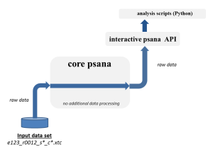
 

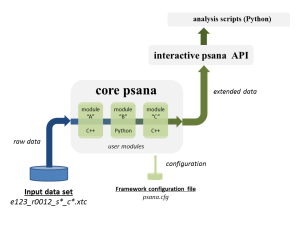
From a prospective of psana python script users, each event read from an input data set will have to go first through a chain of modules before finally getting to the user's script. The events may be modified/extended by the modules as they'll be going along this path. This mechanism is opening a number of interesting possibilities:

• extending an event with derived (processed) data before it will get to the user
• collecting various statistics on the data orthogonal to the top-level analysis algorithm
• combining heavy-weight data processing (by means of the base framework modules written in C++) with the data visualization at the Python framework level

All of this together with a flexibility of the top-level Python scripts allows to build rather powerful data processing/analysis workflows (pipelines, etc.).

However users should be also aware (careful) about certain limitations of the technique in the present version of the framework:

• skipping (filtering) events by the modules won't work. The Python code will be receiving all events read from an input data set.
• re-opening the same data set will result in a complete restart in the internal state of psana modules as if they were run in a separate job after the re-opening.

The rest of this chapter will provide a brief introduction into how to turn on and use the feature in the framework.

Configuring psana to use external modules

External modules are activated in the framework in one of two ways. The most common is a specially prepared configuration file. One can also use Python functions to specify configuration. In both cases, this has to be done before opening a data set. Otherwise the configuration will not apply to the data source that is created. Here is an example that uses a configuration file:

cfg = "/reg/g/psdm/tutorials/cxi/cspad_imaging/frame_reco.cfg"
setConfigFile(cfg)
ds = DataSource('exp=CXI/cxitut13:run=22')

Also note that the core psana also allows an optional data set specification to be placed into the configuration files. This specification will be ignored by the psana python script where the data set is required to be explicitly passed into function DataSource() as a positional parameter. Please, read the Psana User Manual for further instructions on how to write the configuration files.

Here is an equivalent example using the Python function setOptions to set the configuration using one Python dictionary:

cfg = { 'psana.modules':'CSPadPixCoords.CSPadImageProducer',
        'CSPadPixCoords.CSPadImageProducer.source':'CxiDs1.0:Cspad.0',
        'CSPadPixCoords.CSPadImageProducer.typeGroupName':'CsPad::CalibV1',
	    'CSPadPixCoords.CSPadImageProducer.key':'',
	    'CSPadPixCoords.CSPadImageProducer.imgkey':'reconstructed',
        'CSPadPixCoords.CSPadImageProducer.tiltIsApplied':True,
        'CSPadPixCoords.CSPadImageProducer.print_bits':0}
setOptions(cfg)
ds = DataSource('exp=CXI/cxitut13:run=22')

The other Python function for setting options is setOption, for setting an individual option. One could use this in conjunction with setConfigFile. For example:

cfg = "/reg/g/psdm/tutorials/cxi/cspad_imaging/frame_reco.cfg"
setConfigFile(cfg)
setOption('CSPadPixCoords.CSPadImageProducer.print_bits',3)
 ds = DataSource('exp=CXI/cxitut13:run=22')

where the call to setOption overrides the value given for print_bits in the config file.

Module Configuration Parameters

Module configuration parameters can be set within python using commands like:

setOption('psana.allow-corrupt-epics',True)

If you write your own python module, you can access your own module configuration parameters.  This example would load a boolean named 'doSubtraction', which defaults to 'True' if not present in the .cfg file:

self.doSubtraction = self.configBool('doSubtraction', True)

The full list of usable functions is:

configBool
configInt
configFloat
configStr
configSrc
configListBool
configListFloat
configListStr
configListSrc

Calibration modules example: re-constructing a full CSPad image

In this section we're going to explore in a little bit more details the effect of the configuration file which was used in the previous. First, let's have a look at the contents of that file:

[psana]
verbose         = 0
modules         = CSPadPixCoords.CSPadImageProducer

[CSPadPixCoords.CSPadImageProducer]

source          = CxiDs1.0:Cspad.0
typeGroupName   = CsPad::CalibV1
key             =
imgkey          = reconstructed
tiltIsApplied   = true
print_bits      = 0

This configuration refers to some real module (CSPadImageProducer from the OFFLINE Analysis package CSPadPixCoords) which will be doing the geometric reconstruction of the full CSPad image. This module is a part of any latest analysis releases. The main effect of the module is that it will extend each event by an additional component which otherwise wouldn't be present in the event (look for the first one in the output below):

evt.keys()
..
EventKey(type=psana.ndarray_int16_2, src='DetInfo(CxiDs1.0:Cspad.0)', key='reconstructed'),
..
EventKey(type=psana.CsPad.DataV2, src='DetInfo(CxiDsd.0:Cspad.0)'),
..

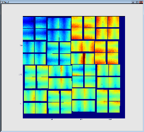
That component has an additional key='reconstructed' (please, refer back to the section on the Four forms of the get() method for more information on that parameter). An object returned with that key has a type of a 2D array of 16-bit elements representing CSPad pixels. With a little bit of help from Matplotlib one can easily turn this into an image. The next example will illustrate how to show both raw (unprocessed) and reconstructed version of the CSPad image:

import matplotlib.pyplot as plt

plt.figure()
plt.ion()
plt.show()

cspad = evt.get(CsPad.DataV2,Source('DetInfo(CxiDs1.0:Cspad.0)'))
a = []
for i in range(0,4):
    quad = cspad.quads(i)
    d = quad.data()
    a.append(np.vstack([d[i] for i in range(0,8)]))

frame_raw = np.hstack(a)

frame_reconstructed = evt.get(ndarray_int16_2,Source('DetInfo(CxiDs1.0:Cspad.0)'),'reconstructed')

plt.imshow(frame_raw)
plt.clim(850,1200)

plt.imshow(frame_reconstructed)
plt.clim(850,1200)

The result is shown below. The first (on the left) image represents 32 so called 2x1 CSpad elements stacked into a 2D array. The second images represents a geometrically correct (including relative alignment of the elements) frame: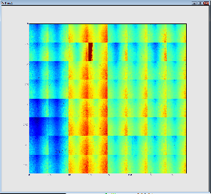
 

Advanced Topics

Random Access to XTC Files ("Indexing")

Individual events can be randomly accessed with code similar to the following:

import psana
# note the "idx" input source at the end of this line: indicates that events will be accessed randomly.
ds = psana.DataSource('exp=xcstut13:run=15:idx')
for run in ds.runs():
    # get array of timestamps of events and iterate over them in reverse order
    times = run.times()
    for tm in times[11:3:-2]:
        evt = run.event(tm)
        print "event id: ", evt.get(psana.EventId)

The events within a calibration-cycle ("step") can be randomly accessed similarly, but using lines like this to get the appropriate times:

nsteps = run.nsteps()
for i in range(nsteps):
    times = run.times(i)

Some notes about indexing:

• If you have a list of timestamps for some other analysis, those can be used in the run.event() method without using the run.times() method.
• Index files are only made available by the DAQ at the end of the run, so can be used before then (this makes "realtime" FFB/shared-memory analysis impossible.
• Indexing only currently works with XTC files (no HDF5 support)
• Currently, indexing only has information about one run at a time (one cannot easily jump between events in different runs).

MPI Parallelization

Using the above indexing feature, it is possible to use MPI to have offline-psana analyze events in parallel (this is useful for many, but not all, algorithms) by having different cores access different events (up to "thousands" of cores).  MPI can also work for online-psana from shared memory (an example script is here that was able to process 120Hz with 7MB/event on 3 machines (8 cores per machine)). See Shared Memory Notes (limited access internal reference) when issues arise.  Online-psana from FFB can only be parallelized using MPI up to the number of DAQ "streams" (typically 6).  For an experiment that wants to use this parallelization: it's a good idea to increase the archiving rate of the slow EPICS data to the shot-rate.

This is some offline-psana sample code that sums a few images in parallel using the indexing feature:

import psana
import numpy as np
import sys
from mpi4py import MPI
comm = MPI.COMM_WORLD
rank = comm.Get_rank()
size = comm.Get_size()
ds = psana.DataSource('exp=XCS/xcstut13:run=15:idx')
src = psana.Source('DetInfo(XcsBeamline.0:Princeton.0)')
maxEventsPerNode=2
for run in ds.runs():
    times = run.times()
    mylength = len(times)/size
    if mylength>maxEventsPerNode: mylength=maxEventsPerNode
    # this line selects a subset of events, so each cpu-core ("rank") works on a separate set of events
    mytimes= times[rank*mylength:(rank+1)*mylength]
    for i in range(mylength):
        evt = run.event(mytimes[i])
        if evt is None:
            print '*** event fetch failed'
            continue
        cam = evt.get(psana.Princeton.FrameV1,src)
        if cam is None:
            print '*** failed to get cam'
            continue
        if 'sum' in locals():
            sum+=cam.data()
        else:
            sum=cam.data().astype(float)
        id = evt.get(psana.EventId)
        print 'rank',rank,'analyzed event with fiducials',id.fiducials()
        print 'image:\n',cam.data()
sumall = np.empty_like(sum)
#sum the images across mpi cores
comm.Reduce(sum,sumall)
if rank==0:
    print 'sum is:\n',sum all
MPI.Finalize()

This can be run interactively by saving the above script in a file called mpi.py and parallelizing the analysis over 2 cores with the commands:

mpirun -n 2 python mpi.py

or run in a batch job:

bsub -a mympi -n 2 -o mpi.log -q psanacsq python mpi.py

The above will run both cores of the job on one node.  If you want the cores to run on different nodes (e.g. to increase available I/O bandwidth) add the following option to the bsub command:

-R "span[ptile=1]"

More examples of using mpi4py can be found at http://mpi4py.scipy.org/docs/usrman/tutorial.html and a broader view of the capabilities of mpi can be found at http://www.open-mpi.org/doc/v1.8/.  Philip Hart also recommended these two links: http://www.sagemath.org/doc/numerical_sage/mpi4py.html, https://computing.llnl.gov/tutorials/mpi/.

Real-time Online Plotting/Monitoring

psana-python code can be run both offline and online (from shared memory, or the Fast-FeedBack (FFB) disks).  Dan Damiani and Ankush Mitra have written software that makes online plotting available based on pyqtgraph (for display) and zeromq (for transferring display data on the network).  This is some example psana-python code that does both a one and a two dimensional plot of numpy arrays (more complex examples, including plot overlays etc. can be found in /reg/g/psdm/sw/releases/ana-current/psmon/examples/).  The last 4 lines are the only lines directly relevant to the plotting (everything else is standard psana-python):

from psana import *
from psmon import publish
from psmon.plots import XYPlot,Image
import sys
ds = DataSource('exp=cxitut13:run=22')
acqsrc  =Source('DetInfo(CxiEndstation.0:Acqiris.0)')
pulnixsrc  =Source('DetInfo(CxiDg4.0:Tm6740.0)')
nbad = 0
ngood = 0
for evt in ds.events():
    if (nbad+ngood)%10 == 0:
        print 'nbad',nbad,'ngood',ngood
    acq = evt.get(Acqiris.DataDescV1,acqsrc)
    pulnix = evt.get(Camera.FrameV1,pulnixsrc)
    if acq == None or pulnix is None:
        nbad+=1
        continue
    ngood+=1
    acqnumchannels = acq.data_shape()
    chan=0
    wf = acq.data(chan).waveforms()[0]
    if (nbad+ngood)%10 == 0:
        ax = range(0,len(wf))
        acqSingleTrace = XYPlot(ngood, "ACQIRIS SINGLE TRACE", ax, wf) # make a 1D plot
        publish.send("ACQSINGLETRACE", acqSingleTrace) # send to the display
        cam = Image(ngood, "Pulnix", pulnix.data16()) # make a 2D plot
        publish.send("PULNIX", cam) # send to the display

The plots can be display with commands like:

psplot -s psanacs031 -p 12301 ACQSINGLETRACE PULNIX

where the "-s" argument is the name of the machine running the above psana-python script, and the "-p" argument is the port number (12301 is the default, but can be overridden with an optional call to publish.init(post=NNNNN)).  If you see this warning from the server:

>[WARNING ] Unable to bind publisher to data port: 12301

it means that there is another server" running on the node that is using up the default network "port number".  If you have an old publisher running, you can kill it using "kill <processId>" where "processId" can be found from the "ps" command.  Alternatively, the publisher should report what port it can use, and then you can specify that port number the -p option to psplot.

It's also possible to plot within 1 python script (no separate "psplot" command necessary) by telling publish to display in a "local" mode:

publish.local = True
# now publish in the usual way
img = Image(0, "Random 1k image", np.random.randn(1024,1024)) 
publish.send('image', img) 

Multiple plots can become "out of synch" (display data for different events).  It is possible to create a "MultiPlot" where the data for all plots stay in synch:

# you can view these plots with a command similar to:
# "psplot -s psanacs057 MULTI"
import psana
from psmon import publish
from psmon.plots import XYPlot, MultiPlot
import numpy as np
import time
def main():
    x = np.linspace(0, np.pi*2, 100)
    for i in range(100):
        y = np.sin(x + np.pi/10*i)
        multi = MultiPlot(i, 'Some Plots')
        sinPlot = XYPlot(i, 'a sine plot', x, y, formats='bs')
        multi.add(sinPlot)
        multi.add(sinPlot)
        publish.send('MULTI', multi)
        time.sleep(0.4)

Dan also writes about how to control the display of the MultiPlot objects:

The MultiPlot class has a field ncols that specifies the number of columns to use when displaying the plots.
It's a keyword in the class constructor.


Also if you want each part of the MultiPlot displayed in separate window (but still synced of course) then pass use_windows=True to the constructor. This one only works for the pyqtgraph client. The ncols one works for both pyqtgraph/matplotlib clients.

Dan has implemented a "matplotlib-style" format string which controls the line/marker shape/color like this:

sinPlot = XYPlot(i, 'a sine plot', x, y, formats='bs')

'bs' means Blue Square. Another example: 'r-' which means red line. Not all matplotlib styles are supported by pyqtgraph, but many are:  http://matplotlib.org/api/pyplot_api.html#matplotlib.pyplot.plot

Minimizing Display Latency

psplot has a buffer size option  (array size that holds the messages on both the display/server side).  This is called the "high water mark" in ZMQ documentation. For the display side use this option to psplot (from the output of "psplot --help"):

-b BUFFER, --buffer BUFFER
the size in messages of receive buffer (default: 10)

For the server side (psana-code):

publish.init(bufsize=2)

Calling C++ from Python using BOOST

This makes use of "ndarray converter" software written by Ankush Mitra which allows you to send numpy arrays between C++/python.  In your psana package, create a subdirectory called "pyext".  In it, include BOOST-style python code (tutorial is Here) similar to this:

#include <boost/python.hpp>
#include <boost/python/overloads.hpp>
#include <boost/python/suite/indexing/vector_indexing_suite.hpp>
#include <pdscalibdata/NDArrIOV1.h>
#include <string>
using namespace boost::python;
typedef pdscalibdata::NDArrIOV1<double,2> MyNDArrIOV1;
BOOST_PYTHON_MEMBER_FUNCTION_OVERLOADS(get_overloads, MyNDArrIOV1::get_ndarray, 0, 1)
BOOST_PYTHON_MEMBER_FUNCTION_OVERLOADS(put_overloads, MyNDArrIOV1::put_ndarray, 1, 2)
BOOST_PYTHON_MODULE(pdscalibdata_pyext)
{
  typedef std::vector<std::string> MyList;
  class_<MyList>("MyList")
    .def(boost::python::vector_indexing_suite<MyList>() );
  class_<MyNDArrIOV1,boost::noncopyable>("NDArrIOV1",init<const std::string &>())
    .def("get_ndarray",&pdscalibdata::NDArrIOV1<double,2>::get_ndarray,get_overloads())
    .def("put_ndarray",&pdscalibdata::NDArrIOV1<double,2>::put_ndarray,put_overloads())
  ;
}

 Note: You need to modify SConscript in your package something like this, to prevent library name conflicts between the BOOST python extension, and the library created by your package:

standardSConscript(PYEXTMOD="pdscalibdata_pyext")

Then you will "import pdscalibdata_pyext" from python.

Re-opening data sets, opening multiple data sets simultaneously

The underlying implementation of the psana framework would create a separate instance of the framework upon each successful call to function DataSource(). This opens two possibilities:

• having many data sets open at a time. All iterations within each instance will be totally independent from others
• re-opening the same dataset. This technique may be useful in case if one wanted to restart the iterators and to start over exploring a data set. Just be careful about the memory management. Python is a dynamic language which has its own garbage collection for objects. Hence if the user code stored (for example - event) references from a prior attempt to open the same dataset then the original instance of the framework will be still around in a process's memory. Under certain circumstances this may result in memory leaks.

The only caveat with making multiple calls to the DataSource() method is that the very last call to the setConfigFile() operation will affect any instances of the framework open with DataSource(). In other words, an order in which functions setConfigFile() and DataSource() does matter. Consider the following example:

ds1 = DataSource(dsname1)   ## no configuration is assumed

setConfigFile('c1.cfg')

ds2 = DataSource(dsname2)   ## the dataset will be processed with c1.cfg
ds3 = DataSource(dsname3)   ## the dataset will be also processed with c1.cfg

setConfigFile('c2.cfg')

ds4 = DataSource(dsname4)   ## the dataset will be processed with c2.cfg
...

Re-opening a dataset is no different from opening multiple different data sets:

ds = DataSource(dsname)

for evt in ds.events():
    ...

ds = DataSource(dsname)     ## this is a fresh dataset object in which
                            ## all iterators are poised to the very first event (run, step)

Working with many events at a time

Unlike its batch version, the psana python script allows multiple events to be present at a time within the process memory. Consider the following extreme scenario:

ds = DataSource(dsname)

events = [evt for evt in ds.events()]

## Now all events are in memory, hence they can be addressed directly
## from the list

evt = events[123]
print evt.run()

However, if you aren't so lucky, and a machine doesn't have enough memory then you would see the run-time exception:

RuntimeError: St9bad_alloc

The second thing to worry about is to make sure all relevant environment data are properly handled. In particular, the event environment objects should be obtained and stored along with each cached event at the same time the event object is retrieved from a dataset and before moving to the next event. The problem was already mentioned in this document when discussing the EPICS Store. As an illustration, let's suppose we need to compare images stored in each pair of consecutive events for all events in a run, and to do the comparison we also need the corresponding values of some PV. In that case the correct algorithm may look like this:

ds = DataSource('exp=XCS/xcstut13:run=15')
epics = ds.env().epicsStore()

prev_evt = None
prev_pv  = None
for evt in ds.events()
    pv = epics.value('LAS:FS0:ACOU:amp_rf1_17_2:rd')
    if prev_evt  is not None:
        ...  ## compare (prev_evt,pv) vs (evt,pv)
    prev_evt = evt
    prev_pv  = pv

APPENDIX

Glossary of Terms

Here is an explanation of terms which are used throughout the document. Some of them have a specific meaning in a context of the Framework and its API:

• data set (or dataset) - a collection of files associated with a run or many runs
• event - a collection of information associated with a particular X-Ray shot at LCLS. Please, note that event is also a Python object in psana.
• environment (or event environment) - a collection of supplementary information which is needed to interpret event data in the right context. It includes: the latest state of the EPICS variables at a time when the event was recorded by the DAQ system, the DAQ configuration information, the calibrations for the instrument's detectors.
• run - a continuous period of time when the DAQ system was running and recording data.
• step (or Calibration Cycle) - an interval within a run when certain experimental environment was stable (such as motor positions, temperatures, etc.)
• detector - a measuring device within an LCLS instrument. This is just a generalization for sensors, diodes, cameras, etc. Can be also known in this document as an event component.
• source - is an object withing the framework's event representing a particular detector
• XTC - is a raw data format for files produced by the LCLS DAQ system. The information is stored in these files sequentially. This implies certain limitation on how various data can be extracted from the files. The files have extension of '.xtc'.
• HDF5 - is a portable data format for files which are produced as a result of translating the raw XTC files. The files have extension of '.h5'.
• PV - Process Variables: typically used to store slowly changing values like voltages/temperatures.  Created by the EPICS control-system software.
• EPICS - Experimental Physics and Industrial Control System, see also Wikipedia
• EVR - Event Receiver.  Electronics that is part of the LCLS timing system that receives shot-to-shot information.  Controls detector triggering and shot-to-shot control of various devices (e.g. pump lasers, shutters)
• MPI - Open MPI  - open source Message Passing Interface implementation, used for analyzing data in parallel on multiple nodes/cores.