Introduction
This is a project suggested by Bebo White to build a PingER monitoring host based on an inexpensive piece of hardware called Raspberry Pi (see more about Raspberry Pi) using a linux distribution as OS (see more about Raspbian). If successful one could consider using these in production reducing the costs, power drain (they draw about 2W of 5V DC power compared to typically over 100W for a deskside computer or 20W for a laptop) and space (credit card size) assisting monitoring sites to be able to procure and support such monitoring hosts. This could be very valuable for sites in developing countries where cost, power utilization and to a lesser extent space may be crucial.
PingER
PingER (Ping End-to-end Reporting) is the name given to the Internet End-to-end Performance Measurement (IEPM) project to monitor end-to-end performance of Internet links. It is led by SLAC and development includes NUST/SEECS (formerly NIIT), FNAL, and ICTP/Trieste, together with UM,UNIMAS and UTM in Malaysia. Originally, in 1995 it was for the High Energy Physics community, however, this century it has been more focused on measuring the Digital Divide from an Internet Performance viewpoint. The project now involves measurements to over 700 sites in over 160 countries, and we are actively seeking new sites to monitor and monitoring sites for this project, as well as people interested in our data. It uses the ubiquitous ping facility so no special software has to be installed on the targets.
Measurements are made by ~60 measurement Agents (MAs) in 23 countries. They make measurements to over 700 targets in ~ 160 countries containing more than 99% of the world's connected population. The measurement cycle is scheduled at roughly 30 minute intervals. At each measurement cycle, each MA issues a set of pings to each target, stopping when it receives 10 ping responses or it has issued 30 ping requests. From each set of pings one can derive various metrics such as minimum (Min) ping Round Trip Time (RTT) response, average (Avg) RTT, maximum (Max) RTT, standard deviation (Stdev) of RTTs, 25% probability of RTT, 75% probability of RTT, Inter Quartile Range (IQR, )loss, reachability (host is unreachable if get 100 % loss).
The data is publicly available and since the online data goes back to January 1998, it provides 19 years of historical data.
Raspberry Pi Model and Specifications
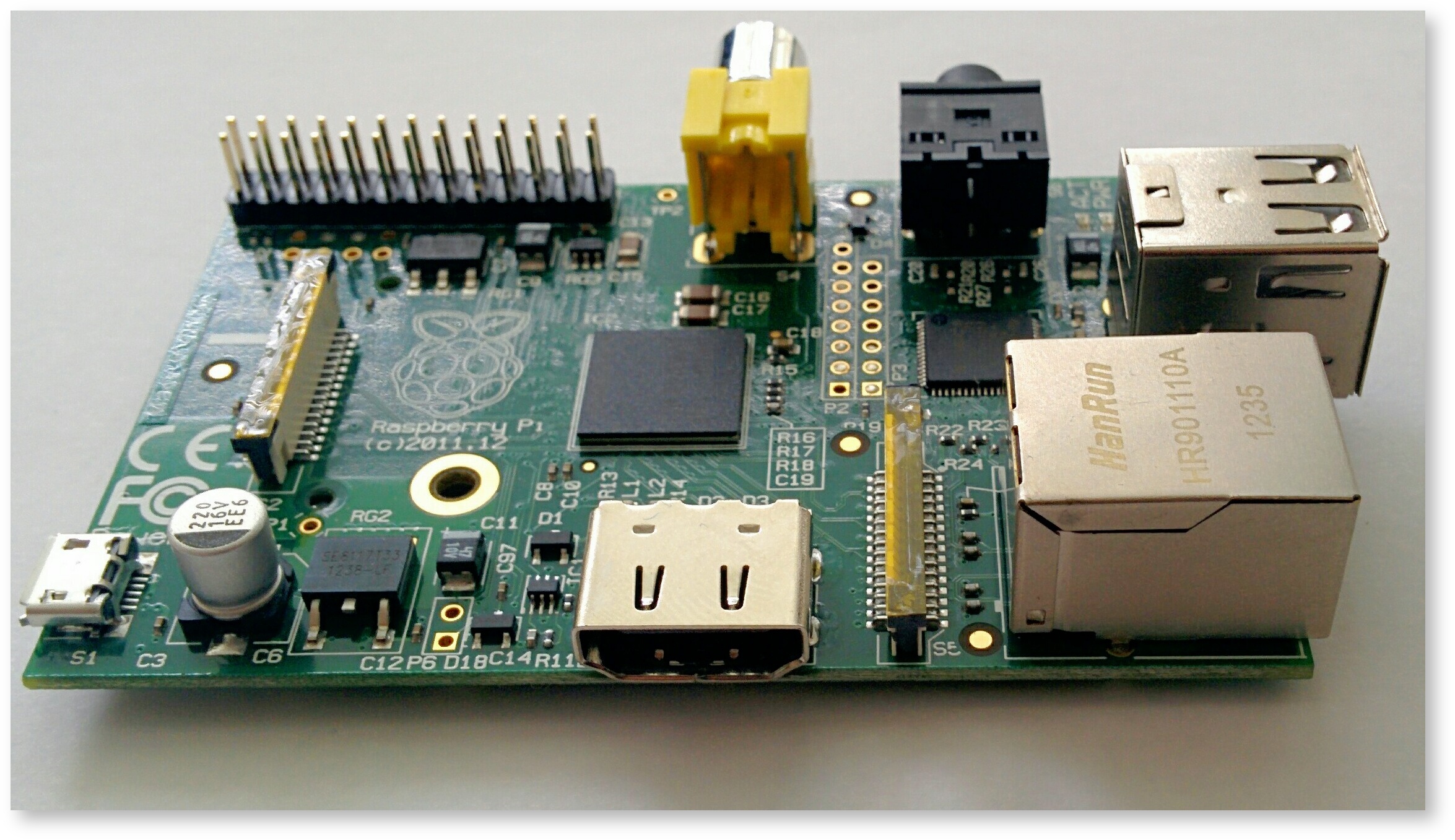
The Raspberry belongs to Bebo White and it is the version 1 of Raspberry Pi, model B. The cost is about $25/each + costs of the SD card. The Raspberry purchased each has 512MB RAM, on a 700Mhz ARM CPU and a 32GB SD Card ($18) was used. They have 2 USB ports and 1 100Mb/s Ethernet interfaces and 1 HDMI port. For reasons of economy it also does not have a Real Time Clock (RTC). Instead, the Pi is intended to be connected to the Internet via Ethernet or WiFi, updating the time automatically from the global ntp (nework time protocol) servers (see https://learn.adafruit.com/adding-a-real-time-clock-to-raspberry-pi/overview). Keep in mind that it is necessary to have a keyboard, a mouse and a HDMI monitor to do the installation process, but once PingER is working they are not necessary anymore. We measured the power (Wattage) during normal use and it is 2.7 Watts. When using the Dell mouse with an LED powered from the Raspberry Pi it crept up to 3.2Watts.
Operating System
The installed system is called Raspbian a Debian Linux variant. The OS had Perl, Make, dig, ping and mail installed. We accessed it through the graphic interface of Raspbian. We just had to install: Apache and XML::Simple.
Installation of PingER2 MA on Raspberry Pi
The first step, before start the installation process we had to change the hostname in Raspbian.
sudo nano /etc/hostname
sudo /etc/init.d/hostname.sh
Notice that the hostname here must include the domain. So, our hostname was pinger.raspberry.slac.stanford.edu.
Then, we followed the instructions in PingER End-to-end Reporting version 2. After installing the PingER2 monitoring code, we installed the ping_data gathering agent, the traceroute server and the pinger_trimmer following the instructions.
When we tested everything, we got a error message on the pingerCronStat.stderr file telling us that the ParserDetails.ini file was missing. We used this approach to fix this.
We entered the machines as monitors in the PingER meta data base of hosts.
Obs: Make sure to change the default password for Raspbian.
Measurements
We chose to make detailed measurements from two monitors at SLAC.
The Dell Poweredge 2650 bare metal pinger.slac.stanford.edu server running Red Hat Linux 2.6.32-504.8.1.el6.i686
pi@pinger-raspberry ~ $ uname -a
Linux pinger-raspberry.slac.stanford.edu 3.18.11+ #781 PREEMPT Tue Apr 21 18:02:18 BST 2015 armv6l GNU/Linux
The Raspberry Pi pinger-raspberry.slac.stanford.edu an armv61 running Gnu Linux (see above).
103cottrell@pinger:~$uname -a
Linux pinger 2.6.32-504.8.1.el6.i686 #1 SMP Fri Dec 19 12:14:17 EST 2014 i686 i686 i386 GNU/Linux
Both were in the same building at SLAC, i.e. roughly at latitude 37.4190 N, longitude 122.2085 W. The machines are about 30 metres apart or about 0.0003 msec based on the speed of light in fibre.
The measurements were made between pinger.slac.stanford.edu and pinger-raspberry.slac.stanford.edu and from both pinger.slac.stanford.edu and pinger-raspberry.slac.stanford.edu to targets at varying distances and hence varying minimum RTTs from SLAC. The Directivity in the table provide a measure of how direct the route is between the MA and target. The Directivity is given as:
Directivity = great circle distance between MA & target [in km] / (RTT [ms] * 100 [km/ms]
The Directivity is <= of 1, and a value of 1 means the RTT is the same as given by the speed of light in a fibre.
| Host | Lat | Long | Great Circle distance from SLAC | Min RTT (as constrained by speed of light in fibre) | Directivity based on measured min RTT |
|---|---|---|---|---|---|
| pinger.slac.stanford.edu | 37.4190 N | 122.2085 W | 0 km | 0.0003 ms | 0.001 |
| pinger-raspberry.slac.stanford.edu | 37.4190 N | 122.2085 W | 0 km | 0.0003 ms | 0.001 |
| sitka.triumf.ca | 49.2475 N | 123.2308 W | 1319.6 km | 13.196 ms | 0.6 |
| ping.cern.ch | 46.23 N | 6.07 E | 9390.6 km | 93.90 ms | 0.63 |
Analysis
Looking for significant differences in the measurements of the more important metrics (minimum, average, median and jitter of RTT and the loss) measured by PingER that impact applications such as throughput, voice over IP, streaming video, haptics, estimating the geolocation of a host by pinging it from well know landmarks. Such differences might result in significant discontinuities in the metric measurements if we were to change the monitoring host.
In this report the jitter is represented by the Inter Packet Delay (IPD).
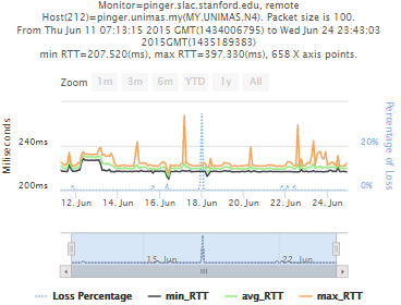
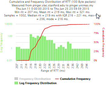
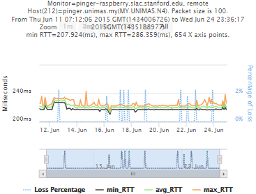
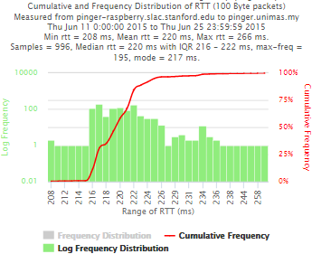
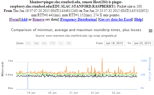
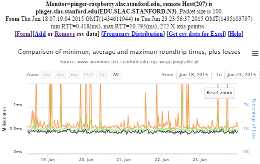
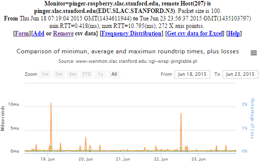
Example target = pinger.unimas.my (~220 msec.)
For both 100Byte and 1000 Byte pings (not shown above) the round trip time series for RTTs have similar behaviour and there are similar losses 7:10 (pinger : pinger-raspberry for 100 Byte pings), note the different Y scales for losses. The losses are about double for 1000Byte pings.
| Time Series | Frequency Distributions |
|---|---|
 |  |
 |  |
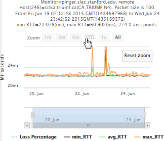
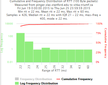
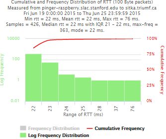
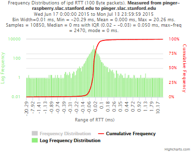
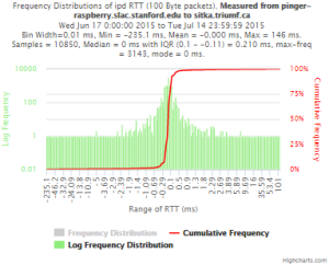
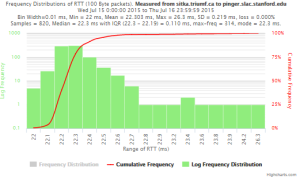
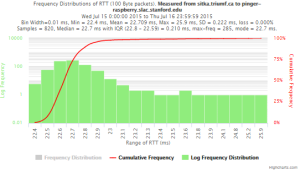
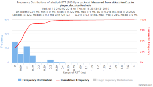
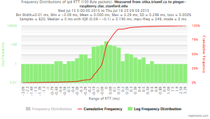
Example target sitka.triumf.ca (~22msec.)
For 100Byte the round trip time series for RTTs did not have similar behaviour. We noticed a great change mainly in the maximum round trip time. The average minimum RTT did not change that much. Another point about pinger-raspberry is that it increases significantly the RTT for near nodes (about ~1ms). The difference is greater than if we compare a node which is in a long distance.
| Time series | Frequency distributions |
|---|---|
 |  |
 |  |
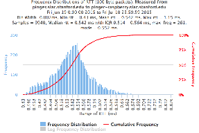
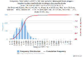
Example between pinger.slac.stanford.edu and pinger-raspberry.slac.stanford.edu
Now, we compared the RTT between pinger and pinger-raspberry. They are located in the same network and the RTT should be very small. However, as noticed before pinger-raspberry has a greater maximum RTT than pinger. The average RTT also has some difference, but now as much as the maximum time has. Note that the second graph represents the third graph using the same scale as the first (pinger graph).
| pinger to Pinger-raspberry | pinger-raspberry to pinger |
|---|---|
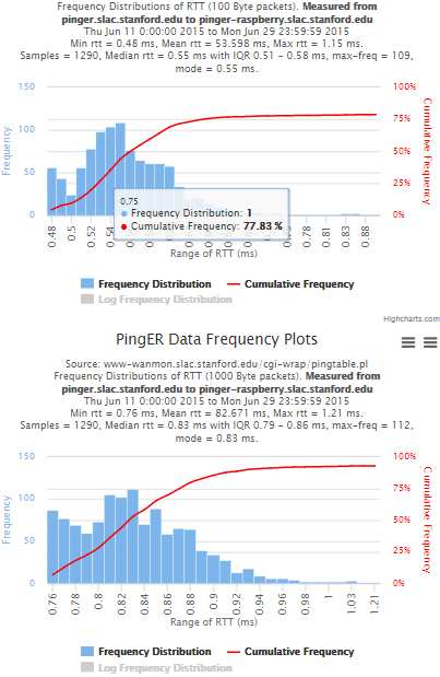 | 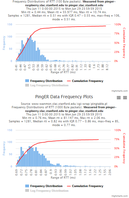 |
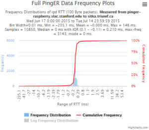
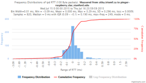
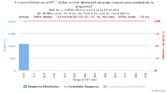
Using full set of pings for RTT frequency distributions
The frequency plots above are for the frequencies of the minimum, average and maximum RTTs. Below we show the frequencies when we take the individual pings (usually 10 assuming little loss) for all the ping RTTs in each measurement set.
| pinger to pinger-raspberry | pinger-raspberry to pinger |
|---|---|
 |  |
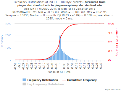
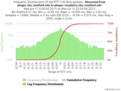
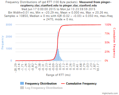
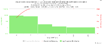
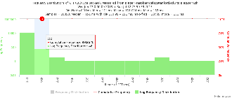
Frequency distribution for absolute interpacket delays.
The magnitude of the RTT is very dependent on the distance of the path between the source and destination. Many applications such as voice over IP, video streaming, or haptics are very dependent on the variability or jitter of the RTT. The jitter is often more dependent on the network edges compared to the RTT. There are many ways to calculate the jitter (see for example http://www.slac.stanford.edu/comp/net/wan-mon/tutorial.html#variable). We calculate the inter packet delay (IPD)and the absolute IPD and display the frequency distributions and statistics.
| pinger to pinger-raspberry | pinger-raspberry to pinger | |
|---|---|---|
| IPD |
|
|
| Abs(IPD) | 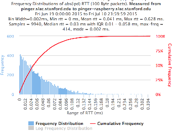 | 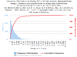 |
To sitka.triumf.ca from SLAC
| pinger.slac.stanford.edu to sitka.triumf.ca | pinger-raspberry.slac.stanford.edu to sitka.triumf.ca | |
|---|---|---|
| Time Series | 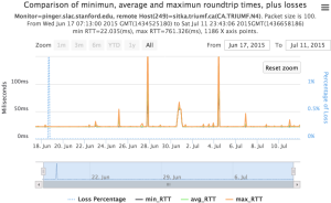 | 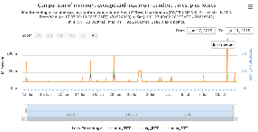 |
| Frequency distribution RTT |  |  |
| Frequency distribution Abs(IPD) | 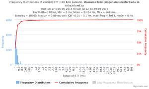 | 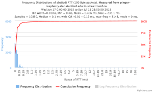 |
| Frequency distribution IPD |
|
|
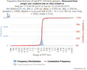
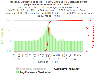
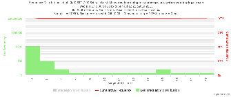
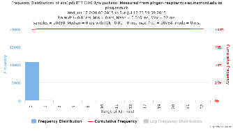
From sitka.triumf.ca to SLAC
| sitka.triumf.ca to pinger.slac.stanford.edu | sitka.triumf.ca to pinger-raspberry.slac.stanford.edu | |
|---|---|---|
| Time series | 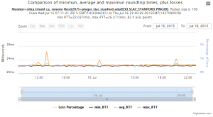 | 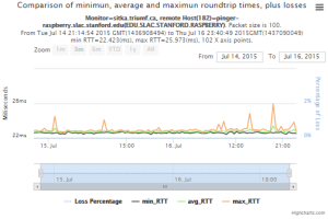 |
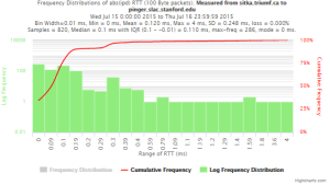
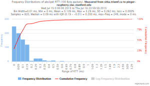
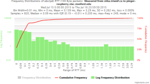
| Frequency Distribution of RTT |
|
|
| Frequency distribution of Abs(IPD) |
|
|
| Frequency distribution of IPD | 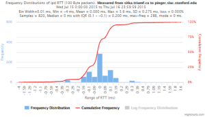 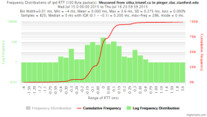 |
|


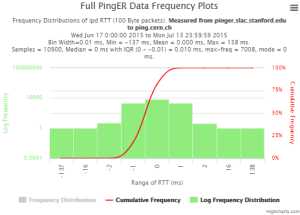
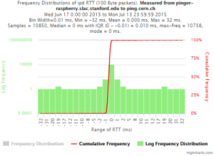
To CERN from SLAC
| To ping.cern.ch from pinger | To ping.cern.ch from pinger-raspberry | |
|---|---|---|
| Time series | 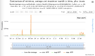 | 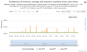 |
| Frequency Distribution RTT |
|   |
Frequency Distribution Abs(IPD) |
 |
 |
| Frequency Distribution IPD |
|
|


Summary
The table below shows the various aggregate metrics measured from monitor to target comparing pinger.slac.stanford with pinger-raspberry.slac.stanford.edu. The columns are arranged in pairs. The first of each pair is for pingerr.slac.stanford.edu, the second for pinger-raspberry.slac.stanford.edu. Each pair is measured over the same time period. Different pairs are measured over different time periods.
| Metric \ Monitor Target | pinger to pinger-raspberry | pinger-raspberry to pinger | pinger to sitka | pinger-raspberry to sitka | sitka to pinger | sitka to pinger-raspberry | pinger to CERN | pinger-raspberry to CERN |
|---|---|---|---|---|---|---|---|---|
| Time period | July 15 - July 16 2015 | July 15 - July 16 2015 | ||||||
| Samples | 820 | 820 | ||||||
Min RTT | 0.43 ms | 0.41 ms | 22 ms | 22.3 ms | 22 ms | 22.4 ms | 150 ms | 151 ms |
| Avg RTT | 0.542 ms | 0.529 ms | 23.9 ms | 23.827 ms | 22.303 ms | 22.709 ms | 150.307 ms | 151.024 ms |
Max RTT | 1.15 ms | 20.8 ms | 761 ms | 334 ms | 26.3 ms | 25.9 ms | 288 ms | 183 ms |
| Stdev | 0.055 ms | 0.540 ms | 9.58 ms | 9.60 ms | 0.219 ms | 0.222 ms | 9.572 ms | 9.594 ms |
| Median RTT | 0.542 ms | 0.51 ms | 22.3 ms | 22.7 ms | 22.3 ms | 22.7 ms | 150 ms | 151 ms |
| 25% | 0.514 ms | 0.48 ms | 22.2 ms | 22.69 ms | 22.3 ms | 22.8 ms | 149.99 ms | 150.99 ms |
| 75% | 0.564 ms | 0.532 ms | 22.4 ms | 22.8 ms | 22.19 ms | 22.59 ms | 151 ms | 151 ms |
| IQR | 0.05 ms | 0.052 ms | 0.2 ms | 0.11 ms | 0.113 ms | 0.210 ms | 1.01 ms | 0.01 ms |
| Min IPD | -0.59 ms | -20.29 ms | -244 ms | -235.1 ms | -0.4 ms | -0.39 ms | -137 ms | -32 ms |
| Avg IPD | 0 ms | 0 ms | 0 ms | 0 ms | 0 ms | 0 ms | 0 ms | 0 |
| Max IPD | 0.62 ms | 20.26 ms | 268 ms | 146 ms | 3.6 ms | 3.29 ms | 138 ms | 32 ms |
| Median IPD | 0 ms | 0 ms | 0 ms | 0 ms | 0 ms | 0 ms | 0 ms | 0 ms |
| Stdev | 0.248 ms | 0.296 ms | ||||||
| 25% IPD | -0.04 ms | -0.03 ms | -0.1 ms | -0.11 ms | -0.1 ms | -0.1 ms | -0.01 ms | -0.01 ms |
| 75% IPD | 0.03 ms | 0.02 ms | 0.09 ms | 0.1 ms | 0.01 ms | 0.09 ms | 0 ms | 0 ms |
| IQR IPD | 0.07 ms | 0.05 ms | 0.190 ms | 0.210 ms | 0.2 ms | 0.190ms | 0.01 ms | 0.01 ms |
| Min(abs(IPD)) | 0 ms | 0 ms | 0 ms | 0 ms | 0 ms | 0 ms | 0 ms | 0 ms |
| Avg(abs(IPD)) | 0.041 ms | 0.066 ms | 0.424 ms | 0.406 ms | 0.120 ms | 0.139 ms | 0.386 ms | 0.046 ms |
| Max(abs(IPD)) | 0.0628ms | 20.294 ms | 268 ms | 235.1 ms | 4 ms | 3.29 ms | 138 ms | 32 ms |
| Stdev | 0.248 ms | 0.262 ms | ||||||
| Median(abs(IPD)) | 0.03ms | 0.024 ms | 0.09 ms | 0.1 ms | 0.1 ms | 0.09 ms | 0 ms | 0 ms |
| 25%(abs(IPD)) | 0.01ms | 0.008 ms | 0.01 ms | 0.01 ms | -0.01 ms | -0.01 ms | 0.01 ms | 0.01 ms |
| 75%(abs(IPD)) | 0.058 ms | 0.05 ms | 0.1 ms | 0.19 ms | 0.1 ms | 0.19 ms | 1 ms | 0 ms |
| IQR(abs(IPD) | 0.048 ms | 0.042 ms | 0.09 ms | 0.11 ms | 0.11 ms | 0.2 ms | 0.009 ms | 0.01 ms |
| Loss | 0% | 0% | 0.008% | 0.000% | 0.000% | 0% | 0% |
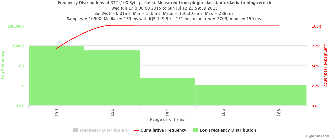
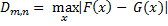
Kolmogorov-Smirnov Test
The Kolmogorov-Smirnov test (KS-test) tries to determine if two datasets differ significantly. The KS-test has the advantage of making no assumption about the distribution of data. In other words it is non-parametric and distribution free. The method is explained here and makes use of an Excel tool called "Real Statiscs". The tests were made using the raw data and distributions, both methods had similar results except for the 100Bytes Packet that had a great difference in the results. The results using raw data says both samples does not come from the same distribution with a significant difference, however if we use distributions the result says that only the 1000Bytes packet does not come from the same distribution. Bellow you will find the graphs for the distributions that were created and the cumulative frequency in both cases plotted one above other (in order to see the difference between the distributions).
| Raw data - 100 Packets | Distribution - 100 Packets | Raw data - 1000 Packets | Distribution - 1000 Packets | |
|---|---|---|---|---|
| D-stat | 0.194674 | 0.039323 | 0.205525 | 0.194379 |
| P-value | 4.57E-14 | 0.551089 | 2.07E-14 | 7.32E-14 |
| D-crit | 0.0667 | 0.067051 | 0.0667 | 0.067051 |
| Size of Raspberry | 816 | 816 | 816 | 816 |
| Size of Pinger | 822 | 822 | 822 | 822 |
| Alpha | 0.05 | |||
If D-stat is greater than D-crit the samples are not considerated from the same distribution with a (1-Alpha) of accuracy. Remember that D-stat is the maximum difference between the two cumulative frequency curves.
Source: http://www.real-statistics.com/non-parametric-tests/two-sample-kolmogorov-smirnov-test/