To World (excluding SLAC targets).
the following tables are from pingtable.pl
Pinger non VM measurement agent
| Tick | min | 25th% | avg | median | 75th% | 90th% | 95th% | max | iqr | std dev | # pairs |
|---|---|---|---|---|---|---|---|---|---|---|---|
| Mar2015 | 23.312 | 178.346 | 239.329 | 211.152 | 293.499 | 339.425 | 379.947 | 780.659 | 115.153 | 104.510 | 107 |
| Feb2015 | 22.689 | 176.167 | 241.608 | 212.435 | 295.448 | 326.637 | 362.350 | 803.815 | 119.281 | 110.212 | 112 |
NB. February data is incomplete for the VM, so leave out
PingER VM measurement agent
| Tick | min | 25th% | avg | median | 75th% | 90th% | 95th% | max | iqr | std dev | # pairs |
|---|---|---|---|---|---|---|---|---|---|---|---|
| Mar2015 | 23.698 | 176.221 | 238.352 | 213.278 | 294.279 | 340.938 | 381.412 | 796.140 | 118.058 | 109.834 | 107 |
| Feb2015 | 22.515 | 178.790 | 239.368 | 210.327 | 301.033 | 329.510 | 369.066 | 807.798 | 122.243 | 110.401 | 110 |
To Europe
PingER non VM Measurement agent
| Tick | min | 25th% | avg | median | 75th% | 90th% | 95th% | max | iqr | std dev | # pairs |
|---|---|---|---|---|---|---|---|---|---|---|---|
| Mar2015 | 150.996 | 162.944 | 175.858 | 173.632 | 186.939 | 201.843 | 204.698 | 204.698 | 23.995 | 17.131 | 14 |
PingER VM Measurement agent
To N. America
PingerVM non VM measurement agent
| Tick | min | 25th% | avg | median | 75th% | 90th% | 95th% | max | iqr | std dev | # pairs |
|---|---|---|---|---|---|---|---|---|---|---|---|
| Mar2015 | 23.312 | . | 54.890 | 62.042 | 79.315 | 79.315 | 79.315 | 79.315 | . | 28.678 | 3 |
PingER VM measurement agent
| Tick | min | 25th% | avg | median | 75th% | 90th% | 95th% | max | iqr | std dev | # pairs |
|---|---|---|---|---|---|---|---|---|---|---|---|
| Mar2015 | 23.095 | 41.357 | 42.888 | 62.077 | 79.350 | 79.350 | 79.350 | 61.775 | 4 |
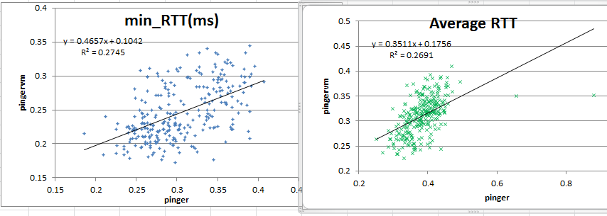
Correlation plots of pinger vs pingervm for hourly measurements
Below are correlation plots of hourly PingER measurements between pinger.slac.stanford.edu and pingervm.slac.stanford.edu between Feb 26 and March 3rd, 2015.
Time series
If one compares the average and median statistics for the tow sets of data, one gets the tables below:
| pinger>pingervm | min_RTT(ms) | avg_RTT(ms) | max_RTT(ms) |
| Average | 0.304368 | 0.385107 | 0.50461 |
| standard deviation | 0.045313 | 0.054924 | 0.272844 |
| median | 0.297 | 0.385 | 0.471 |
| IqR | 0.07625 | 0.0635 | 0.08075 |
| Count | 272 | 272 | 272 |
| pingervm>pinger | min_RTT(ms) | avg_RTT(ms) | max_RTT(ms) |
| Average | 0.245923 | 0.310827 | 0.392096 |
| stdev | 0.040275 | 0.03718 | 0.052863 |
| Median | 0.237 | 0.315 | 0.386 |
| IQR | 0.06425 | 0.04925 | 0.077 |
| Count | 272 | 272 | 272 |
And plots of the time series appears as below (spreadsheet)?
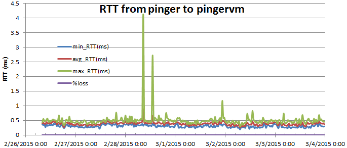
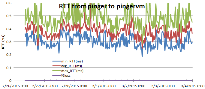
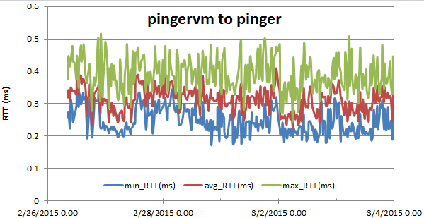
Looking at the above manually scaled plots of pinger>pingervm and pingervm>pinger it is apparent the RTTs from pinger to pingervm are > pingervm to pinger. Looking at the average, standard deviation, median and IQR tables and the differences between pinger as the monitoring site and pingervm as the monitoring site, we see in tabular form (where the average errors are +- (stdev(pinger>pingervm)+stdev(pingervm>pinger)) and the median errors are +- (IQR(pinger>pingervm) + IQR(pingervm>pinger)). the Probabilities are those that the pinger>pingervm and pingervm>pinger distributions are the same (assuming normal distributions).
| Diff (pinger-pingervm) | min_RTT(ms) | +- | Probability | avg_RTT(ms) | +- | Probability | max_RTT(ms) | +- | Probability |
| Average | 0.058445 | 0.085588 | 0.682689 | 0.074279 | 0.092104 | 0.682689 | 0.112515 | 0.325707 | -0.99405 |
| stdev | 0.005037 | 0.017744 | 0.21998 | ||||||
| median | 0.06 | 0.1405 | 0.07 | 0.11275 | 0.085 | 0.15775 | |||
| IqR | 0.012 | 0.01425 | 0.00375 |
It appears that the min_rtts, avg_rtts and max_rtts are within 1 standard deviation (better than 68% assuming a normal distribution) of one another.
By looking at the cumulative distributions we can get the Median differences probability.