Page History
...
The white light, now "imprinted" with the x-ray pulse, is dispersed by a diffraction grating onto a camera. Here's what the raw signal looks like, typically:
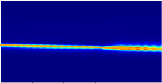
If you take a projection of this image along the y-axis, you obtain a trace similar to this:
...
| Info | ||
|---|---|---|
| ||
| From Matt Weaver 8/23/17: (including extra thoughts transcribed by cpo from Matt on 02/26/20) The spectrum ratio is treated as a waveform, and that waveform is analyzed with a Wiener filter in the "time" domain. It is actually a matched filter where the noise is characterized by taking the ratio of non-exposed spectra from different images - should be flat but the instability of the reference optical spectrum causes it to have correlated movements. So, the procedure for producing those matched filter weights goes like this:
There's a script (http://pswww.slac.stanford.edu/svn-readonly/psdmrepo/TimeTool/trunk/data/timetool_setup.py) which shows the last steps of the calibration process that produces the matched filter weights from the autocorrelation function and the signal waveform. That script has some inputs hard-coded into it, but it at least shows the procedure. It requires some manual intervention to get a sensible answer, since there are often undesirable features in the signal that the algorithm picks up and tries to optimize towards. |
The astute reader will notice that this trace has no etalon wiggles. That is because it has been cleaned up by subtracting an x-ray off shot (BYKICK). Those events have the same etalon effect, but no edge – subtracting them removes the etalon. That's a good thing, because the etalon wiggles would have given this method a little trouble if they were big in amplitude.
So, to summarize, here is what the DAQ analysis code does:
- Extract the TT trace using an ROI + projection
- Subtract the most recent x-ray off (BYKICK) trace
- Convolve the trace with a filter
- Report the position, amplitude, FWHM of the resulting peak
The reported position will be in PIXELS. That is not so useful! To convert to femtoseconds, we need to calibrate the TT.
| Info | ||
|---|---|---|
| ||
The timetool only gives you a small correction to the laser-xray delay. The "nominal" delay is set by the laser, which is phase locked to the x-rays. The timetool measures jitter around that nominal delay. So you should compute the final delay as: delay = nominal_delay + timetool_correction Since different people have different conventions about the sign that corresponds to "pump early" vs. "pump late" you must exercise caution that you are doing the right thing here. Ensure that things are what you think they are. If possible, figure this out before your experiment begins, or early in running, and write it down. Force everyone to use the same conventions. Especially if you are on night shift :). The "nominal delay" should be easily accessible as a PV. Unfortunately, it will vary hutch-to-hutch. Sorry. Ask your beamline scientist or PCDS PoC for help. |
How to get the results
Results can be accessed using the following epics-variables names:
There's a script (https://github.com/lcls-psana/TimeTool/blob/master/data/timetool_setup.py) which shows the last steps of the calibration process that produces the matched filter weights from the autocorrelation function and the signal waveform. That script has the auto-correlation function and averaged-signal hard-coded into it, but it shows the procedure. It requires some manual intervention to get a sensible answer, since there are often undesirable features in the signal that the algorithm picks up and tries to optimize towards. The fundamental formula in that script is weights=scipy.linalg.inv(scipy.linalg.toeplitz(acf))*(averaged_signal). The above procedure optimizes the filter to reject the background. Matt doesn't currently remember a physical picture of why the "toeplitz" formula optimizes the weights to reject background. If one wants to simplify by ignoring the background suppression optimization, the "average signal" (ignoring the background) can also be used as a set of weights for np.convolve. |
The astute reader will notice that this trace has no etalon wiggles. That is because it has been cleaned up by subtracting an x-ray off shot (BYKICK). Those events have the same etalon effect, but no edge – subtracting them removes the etalon. That's a good thing, because the etalon wiggles would have given this method a little trouble if they were big in amplitude.
So, to summarize, here is what the DAQ analysis code does:
- Extract the TT trace using an ROI + projection
- Subtract the most recent x-ray off (BYKICK) trace
- Convolve the trace with a filter
- Report the position, amplitude, FWHM of the resulting peak
The reported position will be in PIXELS. That is not so useful! To convert to femtoseconds, we need to calibrate the TT.
| Info | ||
|---|---|---|
| ||
The timetool only gives you a small correction to the laser-xray delay. The "nominal" delay is set by the laser, which is phase locked to the x-rays. The timetool measures jitter around that nominal delay. So you should compute the final delay as: delay = nominal_delay + timetool_correction Since different people have different conventions about the sign that corresponds to "pump early" vs. "pump late" you must exercise caution that you are doing the right thing here. Ensure that things are what you think they are. If possible, figure this out before your experiment begins, or early in running, and write it down. Force everyone to use the same conventions. Especially if you are on night shift :). The "nominal delay" should be easily accessible as a PV. Unfortunately, it will vary hutch-to-hutch. Sorry. Ask your beamline scientist or PCDS PoC for help. |
How to get the results
Results can be accessed using the following epics-variables names:
| TTSPEC:FLTPOS | the position of the edge, in pixels |
| TTSPEC:AMPL | amplitude of biggest edge found by the filter |
| TTSPEC:FLTPOSFWHM | the FWHM of the edge, in pixels |
| TTSPEC:AMPLNXT | amplitude of second-biggest edge |
| found by the filter, good for rejecting bad fits | |
| TTSPEC:REFAMPL | amplitude of the background "reference" which is subtracted before running the filter algorithm, good for rejecting bad fits |
| TTSPEC:FLTPOS_PS | the position of the edge, in picoseconds, but requires correct calibration constants be put in the DAQ when data is acquired. Few people do this. So be wary. |
These are usually pre-pended by the hutch, so e.g. at XPP they will be "XPP:TTSPEC:FLTPOS". The TT camera (an OPAL) should also be in the datastream.
...
Unfortunately, right now CXI, XPP, and AMO have different methods for doing this calibration. Talk to your beamline scientist about how to do it and process the results.the results.
Conversion from FLTPOS pixels into ps
Once you do this calibration, it should be possible to write a simple function to give you the corrected delay between x-rays and optical laser. For example, the following code snip was used for an experiment at CXI. NOTE THIS MAY CHANGE GIVEN YOUR HUTCH AND CONVENTIONS. But it should be a good starting point ![]() .
.
| Code Block | ||||
|---|---|---|---|---|
| ||||
def relative_time(edge_position):
    """
    Translate edge position into fs (for cxij8816)

    from docs >> fs_result = a + b*x + c*x^2, x is edge position
    """
    a = -0.0013584927458976459
    b =  3.1264188429430901e-06
    c = -1.1172611228659911e-09
    x = tt_pos(evt)
    tt_correction = a + b*x + c*x**2
    time_delay = las_stg(evt)
return -1000*(time_delay + tt_correction) |
Rolling Your Own
Hopefully you now understand how the timetool works, how the DAQ analysis works, and how to access and validate those results. If your DAQ results look unacceptable for some reason, you can try to re-process the timetool signal. If, right now, you are thinking "I need to do that!", you have a general idea of how to go about it. If you need further help, get in touch with the LCLS data analysis group. In general we'd be curious to hear about situations where the DAQ processing does not work and needs improvement.
...
- It is possible to re-run the DAQ algorithm offline in psana, with e.g. different filter weights or other settings. This is documented extensively.
- There is some experimental python code for use in situations where the etalon signal is very strong and screws up the analysis. It also simply re-implements a version of the DAQ analysis in python, rather than C++, which may be easier to customize. This is under active development and should be considered use-at-your-own-risk. Get in touch with TJ Lane <tjlane@slac.stanford.edu> if you think this would be useful for you.
- -own-risk. Get in touch with TJ Lane <tjlane@slac.stanford.edu> if you think this would be useful for you.
References
https://opg.optica.org/oe/fulltext.cfm?uri=oe-19-22-21855&id=223755
https://www.nature.com/articles/nphoton.2013.11
https://opg.optica.org/oe/fulltext.cfm?uri=oe-28-16-23545&id=433772
Overview
Content Tools