Page History
Content
| Table of Contents |
|---|
Code location
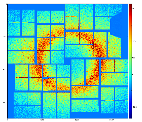
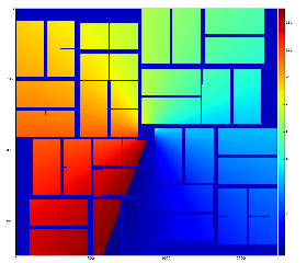
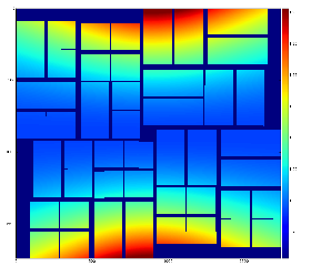
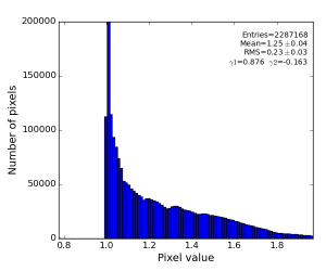
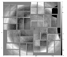
This algorithm is intended to subtract background from "non-assembled" images with approximately angular-symmetric radial distribution of intensities.
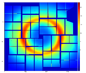
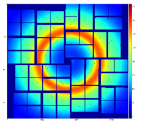
For example, pure water ring background from exp=cxij4716:run=22 for single event has an angular symmetry as shown in the plot:
Code location
Class In LCLS software release code of the class RadialBkgd resides in the package pyimgalgos.
Auto-generated documentation for class RadialBkgd
Initialization
| Code Block |
|---|
from pyimgalgos.RadialBkgd import RadialBkgd, polarization_factor
rb = RadialBkgd(xarr, yarr, mask=None, radedges=None, nradbins=100, phiedges=(0,360), nphibins=32) |
See parameters' description in Auto-generated documentation for class RadialBkgd.
Input n-d arrays can be obtained through the Detector (AreaDetector) interface or directly through the class working with geometre:geometry. For example,
| Code Block |
|---|
from PSCalib.GeometryAccess import GeometryAccess geo = GeometryAccess(fname_geo) xarr, yarr, zarr = geo.get_pixel_coords() iX, iY = geo.get_pixel_coord_indexes() mask = geo.get_pixel_mask(mbits=0377) # mask for 2x1 edges, two central columns, and unbound pixels with their neighbours ... |
Algorithm
Intention
...
For example, pure water ring background from exp=cxij4716:run=22:
To evaluate background in data, n-d array of data is split for 2-d bins in polar coordinate frame, total . Total intensity and number of involved pixels are counted for each bin and converted to the average bin intensity.Then Then this averaged intensity is per-pixel subtracted form from data n-d array.
...
Input per-pixel coordinates passed in as numpy n-d arrays xarr , and yarr are used to evaluate per-pixel radius radial and polar angle coordinate arrays:
| Code Block |
|---|
rad = rb.pixel_rad() phi = rb.pixel_phi() |
Binning parameters radedges, nradbins, phiedges, nphibins are used to initialize 2-d bins using class HBins. Initialization with default binning parameters covers entire detector coordinate space.
...
| Code Block |
|---|
rad = rb.pixel_rad() iseq = rb.pixel_iseq() |
Pixels masked by the n-d array passed in the parameter mask mask are excluded from this algorithm and are not corrected.
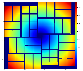
Averaged background intensity for default and (nradbins=200, nphibins=32) and non-default binning cases (nphibins=8, nradbins=500) binning cases :
| Code Block |
|---|
bkgd = rb.bkgd_nda(nda) |
Background subtraction
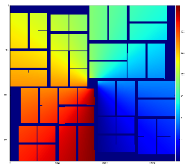
Background subtracted data for default (nradbins=100200, nphibins=32) and non-default binning cases (nradbins=500, nphibins=1), and (nradbins=500, nphibins=8, phiedges=(-20, 240)):
| Code Block |
|---|
res = rb.subtract_bkgd(nda) |
Polarization correction
- For good statistical precision of the background averaging 2-d bins should contain large number of pixels. However large bins produces significant binning artifacts distortion which are seen in resulting image.
- The main reason for angular bins is a variation of intensity with angle due to polarization effect. The beam polarization effect can be eliminated with appropriate correction.
Method for polarization correction factor:
Code Block collapse true def polarization_factor(rad, phi_deg, z) : """Returns per-pixel polarization factors, assuming that detector is perpendicular to Z. """ phi = np.deg2rad(phi_deg) ones = np.ones_like(rad) theta = np.arctan2(rad, z) polsxc = 1 - np.sqrt(np.fabs(np.sin(theta)*np.cos(phi))) pol = 1 - sxc*sxc return divide_protected(ones, pol, vsub_zero=0)
Then, radial background can be estimated for a single angular bins (ringusing ring-shaped radial bins), single bin in angle:
| Code Block |
|---|
arr = load_txt(fname_nda) rb = RadialBkgd(X, Y, mask, nradbins=500, nphibins=1) pf = polarization_factor(rb.pixel_rad(), rb.pixel_phi(), z94e3) resnda = rb.subtract_bkgd(ndaarr * pf) |
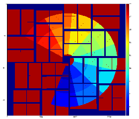
For z=1m we get polarization correction factor, corrected data (water-ring) sample, and background subtracted data as follows.


Effect of polarization is somehow accounted, but most likely the sample-to-detector distance 1m is not correct.
* mask.flatten() |
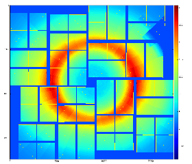
For The data set exp=cxij4716:run=22 was collected at sample-to-detector distance z=94mm. In this case polarization correction formula gives distribution for correction factor and "corrected" data
- averaged over all 14636 events
...
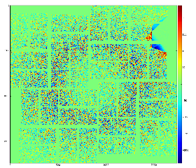
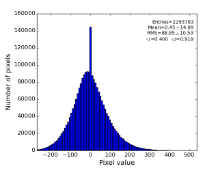
- calibrated (pedestal, common mode) data
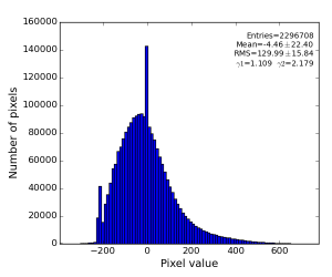
- polarization correction factor
- polarization-corrected data
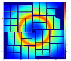
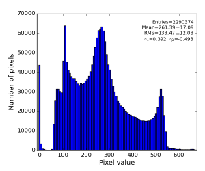
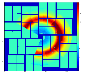
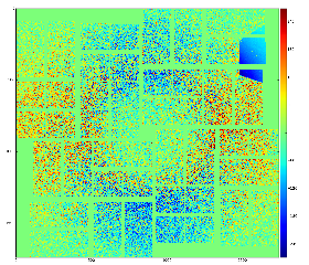
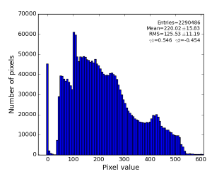
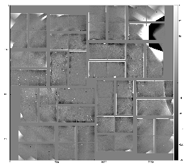
- radial-background subtracted data using single angular bin
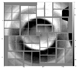
This image indicates on in-correct geometry; background center consistent with beam intersection does not coincide with detector origin (0,0). - radial-background subtracted data using 8 angular bins
dynamically apply some geometry correction
Code Block geo = GeometryAccess(fname_geo) geo.move_geo('CSPAD:V1', 0, 1600, 0, 0) geo.move_geo('QUAD:V1', 2, -100, 0, 0)and plot again radial-background subtracted data using single angular bin
we get that "dish"-like shape disappears.Interpolation (linear) between centers of the background bins could also help:
Code Block bkgd = rb.bkgd_nda_interpol(nda, method='linear') # method='nearest' 'cubic' cdata


So, it looks like polarization correction formula is wrong
CSPAD "dopping" artifacts
...
= rb.subtract_
...
interpol(
...
nda, method='linear')Interpolation for entire detector and for part of the image:
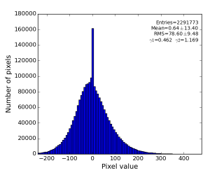
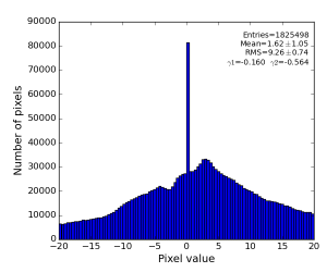
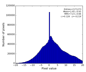
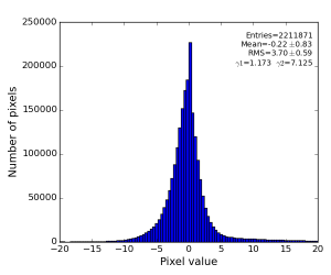
Image is not as impressive as for polarization-corrected sample, but the residual intensity spread shrink down to RMS~3 ADU.
- Single angular bin interpolated background, and its subtraction from data:


CSPAD "dopping" artifacts
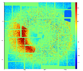
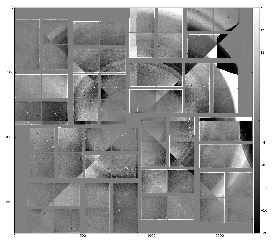
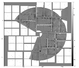
- zoomed-in regions of four quads
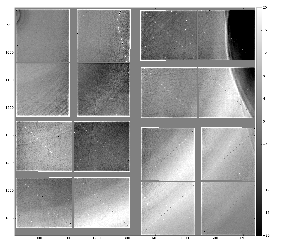
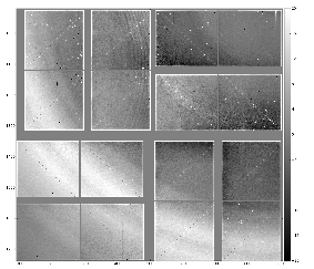
- Shows some "doping" artifacts.
- A few smooth curves earlier interpreted as "scratches" apparently become a nice "chart" probably on the detector shield. This "chart" can be used for alignment.
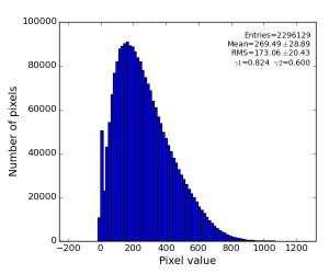
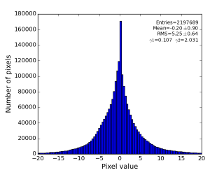
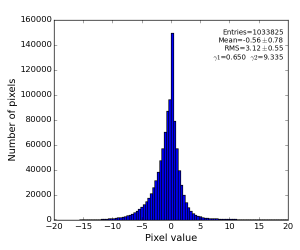
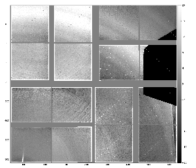
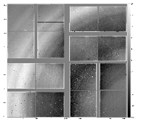
Polarization corrected, radial background subtracted image, array spectra, and zoomed parts of the image with potential artifact candidates:
...
References
Overview
Content Tools