Page History
| Table of Contents |
|---|
Quickstart
The timetool camera measures the time difference between laser and FEL in one of two methods:
- spatial encoding (also called "reflection" mode), where the X-rays change the reflectivity of a material and the laser probesthat change by the incident angle of its wavefront; or
- spectral encoding (also called "transmission" mode), where the X-rays change the transmission of a material and the chirped laser probes it by a change in the spectral components of the transmitted laser.
Both modes can be analyzed with this software, but in "transmission" mode one can typically use the default values for the filter weights (described below). This is because most experiments use a similar setup in this mode. In "reflection" mode, the filter weights must typically be tuned per-experiment, which is a non-trivial task.
TimeTool results can be computed by the DAQ while data is being recorded and written directly into the .xtc files, or after data has been recorded. In AMO/XPP the time tool analysis is done by the DAQ while data is being recorded. Results can be accessed using the following epics-variables names: TTSPEC:AMPL (amplitude of biggest edge found by the filter), TTSPEC:AMPLNXT (amplitude of second-biggest edge found by the filter), TTSPEC:FLTPOS (the position of the edge, in pixels), TTSPEC:FLTPOSFWHM (the FWHM of the edge, in pixels), TTSPEC:FLTPOS_PS (the position of the edge, in picoseconds, but requires correct calibration constants be put in the DAQ when data is acquired), TTSPEC:REFAMPL (amplitude of the background "reference" which is subtracted before running the filter algorithm) or by getting the appropriate Psana.TimeTool.DataV* object from the event (either V1 or V2) from the opal camera source.
| Tip | ||
|---|---|---|
| ||
If you make a plot of the measured timetool delay it is quite noisy (e.g. the laser delay vs. the measured filter position, TTSPEC:FLTPOS, while keeping the TT stage stationary). There are many outliers. This can be greatly cleaned up by filtering based on the TT peak. I (TJ, <tjlane@slac.stanford.edu>) have found the following "vetos" on the data to work well, though they are quite conservative (throw away a decent amount of data). That said they should greatly clean up the TT response and has let me proceed in a "blind" fashion: Require: tt_amp [TTSPEC:AMPL] > 0.05 AND 50.0 < tt_fwhm [TTSPEC:FLTPOSFWHM]< 300.0 This was selected based on one experiment (cxii2415, run 65) and cross-validated against another (cxij8816, run 69). |
This document covers how to run the TimeTool after data has been recorded. Starting with ana-0.16.9, a Python wrapper to the TimeTool is provided which is the preferred way to run the TimeTool algorithms. Previous to ana-0.16.9 one would use Psana modules. One would load the C++ TimeTool.Analyze module via a psana config file.
Note: specific examples for the time tool can be found in /reg/g/psdm/sw/releases/ana-current/TimeTool/examples/.
Python Interface
In the example directory mentioned above, see:
- pyxface_evr_bykick.py
- pyxface_calib_db_ref.py
- control_logic.py
The python interface contains extensive documentation in its docstrings. To access this, from a ipython session, do
| Code Block | ||
|---|---|---|
| ||
import TimeTool

TimeTool.PyAnalyze?
TimeTool.AnalyzeOptions? |
Further documentation can be found on the PyAnalyze functions.
The docstrings will contain the most current documentation. For convenience, we include this documentation here as well:
PyAnalyze
Python interface to the TimeTool.Analyze C++ Psana module to allow conditional execution.
Basic Usage
There are several steps to using the module demonstrated in this example:
| Code Block | ||
|---|---|---|
| ||
ttOptions = TimeTool.AnalyzeOptions(get_key='TSS_OPAL',
                                    eventcode_nobeam = 162)
ttAnalyze = TimeTool.PyAnalyze(ttOptions)
ds = psana.DataSource(self.datasource, module=ttAnalyze)

for evt in ds.events():
ttResults = ttAnalyze.process(evt) |
The steps are
Create an instance of the AnalyzeOptions class. See AnalyzeOptions docstring for detailed documentation on options.
Construct an instance of PyAnalyze (called ttAnalyze above) by passing this options object (called ttOptions above).
construct your psana DataSource by passing the PyAnalyze instance through to the module argument.
call the ttAnalyze.process() method on each event you want to process.
Parallel Processing
When doing parallel processing and distributing events among different ranks, each rank typically processes a fraction of all the events. Howevever it is important that each rank also process all events that include reference shots for the TimeTool. One can check if a shot is a reference shot or not with the isRefShot(evt) function. For example, in the above, suppose the variables numberOfRanks and rank are defined so that we can implement a round robin strategy to distribute event processing. One could implement this, while making sure all ranks process reference shots, as follows:
| Code Block | ||
|---|---|---|
| ||
        for idx, evt in enumerate(ds.events()):
            if ttAnalyze.isRefShot(evt):
                ttAnalyze.process(evt)
            if idx % numberOfRanks != rank:
                continue
ttResults = ttAnalyze.process(evt) |
Note that it is Ok to call the PyAnalyze.process(evt) function more than once on the same event. The PyAnalyze class caches the results of the first call so as to not call the underlying C++ TimeTool.Analyze module twice.
Controlling Beam Logic
This is an unsual use case. It happens when users are using EPICSs to move things around to drop the beam, rather than using an event code, or perhaps they decide that cutting on a Bld parameter will tell them if the laser and beam are interacting or not. But in these cases the user will want to look at the EPICS variables, Bld, or other things, and instruct the TimeTool of when the beam is off so that it can build up its reference.
To do this, do the following:
- set controlLogic=True in AnalyzeOptions
- call the controlLogic(evt, beamOn, laserOn) function for every event that you will have the TimeTool process.
When controlLogic is true, you must call this function for each event you subsequently call process on (if you forget, TimeTool will stop with an error or crash).
Below is a complete example. For the most up to date example, look in the ana-current/TimeTool/examples directory specified above.
| Code Block | ||
|---|---|---|
| ||
import sys
import os
import psana
import TimeTool
from mpi4py import MPI
rank = MPI.COMM_WORLD.Get_rank()
worldsize = MPI.COMM_WORLD.Get_size()
numevents=50
ttOptions = TimeTool.AnalyzeOptions(
    get_key='TSS_OPAL',
    controlLogic=True,        ## KEY STEP
    calib_poly='0 1 0',
    sig_roi_x='0 1023',
    sig_roi_y='425 724',
    ref_avg_fraction=0.5)

ttAnalyze = TimeTool.PyAnalyze(ttOptions)
ds = psana.DataSource('exp=sxri0214:run=158', module=ttAnalyze)
for idx, evt in enumerate(ds.events()):
    if (numevents > 0) and (idx >= numevents): break
    ## when idx is even, we'll call it a reference shot (laser on, but beam off)
    ## and when idx is odd, we'll call it a good shot (both laser and beam on)
    ## however this is where users will insert their own logic based on epics or bld
    if idx % 2 == 0:
        laserOn=True
        beamOn=False
    elif idx % 2 == 1:
        laserOn=True
        beamOn=True
    ttAnalyze.controlLogic(evt, laserOn, beamOn)   ## KEY STEP - call before any call to process
    if ttAnalyze.isRefShot(evt):
        print "rank=%3d event %d is ref shot" % (rank, idx)
        ttAnalyze.process(evt)
    if idx % worldsize != rank:
        continue
    ttdata = ttAnalyze.process(evt)
    if ttdata is None: continue
    print "rank=%3d event %4d has TimeTool results. Peak is at pixel_position=%6.1f with amplitude=%7.5f nxt_amplitude=%7.5f fwhm=%5.1f" % \
                (rank, idx, ttdata.position_pixel(), ttdata.amplitude(), ttdata.nxt_amplitude(), ttdata.position_fwhm())
|
AnalyzeOptions
Specify configuration options for the TimeTool Analyze module.
There are many options for TimeTool.Analyze, most can be left at their default values. First we document options users may want to change, then more specialized options.
Note that all options are either a Python str, or Python int, or float. Even though some options represent a list of numbers, the argument must be formatted as a string with only whitespace separating numbers (no commas, etc).
Common Options
| Code Block |
|---|
    Option    default    data type / explanation
    ------    -------    -----------
    get_key  'TSS_OPAL'  str, this is the psana source for the TimeTool
                         opal camera. The default, 'TSS_OPAL', is a common
                         DAQ alias for this source

    eventcode_nobeam 0   int, for BYKICK experiments, where an evr code
                         specifies when the beam is NOT present, specify that
                         EVR code here. If the beam is always present, keep
                         the default value of 0. Note - there are specialized
                         options to control laser on/off beam on/off logic
                         below.
    ref_avg_fraction 0.05 float, weight assigned to next reference shot in
                          rolling average. 1.0 means replace reference with
                          next shot (no rolling average). 0.05 means next
                          shot is 5% of average and all previous is 95%.
    sig_roi_y '425 725' str, signal roi in y, or the rows of the Opal camera
                         that the user may want to adjust based on where signal is.
    sig_roi_x   '0 1023' str, signal roi in x or columns, default is all.
    calib_poly '0 1 0'   str, TimeTool.Analyze returns results as both a pixel
                         location on the Detector, as well as a conversion
         to femtoseconds by applying this quadratic polynomial. Typically a
         special calibration run is performed to compute the mapping from
         position on the detector to femtoseconds and the results of this
         analysis are passed through this parameter. If calib_poly is 'a b c'
         Then femtosecond_result = a + b*x + c*x^2 wher x is the detector position.
    ** Uncommon Options**
    Option    default    data type / explanation
    ------    -------    -----------
    projectX   True     bool, if true, project down to the X axis of the opal.
    eventcode_skip  0   int, EVR code for events that should be skipped from
                        TimeTool processing.
    ipm_get_key    ''   str, in addition to the evr code above, the timetool
                        will look at the threshold on a specified ipmb to decide
                        if the beam is present. Default is to not look at a
                        ipmb. Here one can specify the psana source for the
                        desired ipimb.

    ipm_beam_threshold  float, threshold for determining if beam present from
                        an ipm.

    weights  '0.00940119 ...' str, this defaults to a long string of the
                        weights that the TimeTool uses when performing signal
                        processing on the normalized, reference divided signal,
                        to turn a sharp drop into a peak. It is unusual for
                        users to modify this string. The full string can be
                        found in the code.
    weights_file ''     str, the weights can be put into a file as well
    use_calib_db_ref  False  bool, get the initial reference from the
                       calibration database. This reference can be deployed
                       using calibman by making a pedestal for the appropriate
                       opal. Example use case is creating references not by
                       dropping the beam from shots, but rather making
                       reference runs (dropped shots tend to give better results).

    ref_load  ''       str, filename to load reference file from.
    ref_store ''       str, filename to store reference into.
    controlLogic      False,  bool, to bypass the normal mechanism of letting
                      the timetool identify when the beam or laser is on,
                      the user can control this. If this is set, then for
                      every event, one must call controlLogic before calling
                      process with the TimeTool.Analyze python class.
    proj_cut   -(1<<31), int, after projecting of the opal camera to create the
                     signal, one can require that at least one value in the signal
                     be greater than this parameter in order to continue processing.
                     Default is int_min, which means one always processes when the
                     laser is on (and a reference is available).
    sb_roi_x   '', str  give something like 1 10 to do sideband analysis and specify
                   the sideband ROI. This feature, while it exists in the code, is not
                   maintained. Experts interested in this feature may need to contact
                   their POC for support.

    sb_roi_y   '', str, see sb_roi_x, this is for the y region (rows)
    sb_avg_fraction 0.05, float, see sb_roi_x and sig_avg_fraction for information on
                    rolling averages.

    analyze_event -1, int, special options for analyzing the first few events with respect
                  to a reference - feature not maintained.
    dump         0, int, setting this option is not reccommended. It instructs TimeTool
                 to use the psana root based historgramming method - however the root
                 files interfere with MPI based analysis. See the eventdump option below
                 to access intermediate stages of TimeTool processing.
    eventdump   False, bool, setting this option to True will cause the underlying C++
                Psana TimeTool.Analyze module to return extra data that the Psana PlotAnalyze
                module can use (or users can get directly) but presently, the Python wrapper
                does not expose this, or setup the plotter in a convenient way. However One can
                get the ndarrays directly from the event following a call to PyAnalyze.Process().
    psanaName TimeTool.Analyze, str, the logging name passed to this instance of the
                underlying C++ Psana Module called TimeTool.Analyze. There should be no
                reason to modify this - unless for some reason you want to configure two
                separate instances of the Psana Module.
    put_key TTANA, str, should be little reason to modify this. This is the key used to get
                 results back from the C++ TimeTool.Analyze module.
    beam_on_off_key ControlLogicBeam, str, there should be no reason to modify this.
                if controlLogic is true, this is the internal key string used to
                communicate beam on/off with the TimeTool.Analyze module.
laser_on_off_key ControlLogicLaser, str, as above, should be no reason to modify this. |
Users migrating older code will need to discard psana config files, or remove the TimeTool.Analyze configuration from the psana config file AS WELL AS THE TimeTool.Analyze C++ Psana Module from the list of psana modules in the config file. If mixing old style Psana modules with PyAnalyze, be advised that PyAnalyze will run after any modules listed in the psana config file (so the TimeTool results will not be available to Psana modules listed in the config file). It should be easy to move Python Psana modules into the new style (C++ modules are not easy to move).
C++ Psana Module Interface
Next we disuss the older, C++ Psana module interface to the TimeTool. The package includes sample configuration files that describe all the options. From a psana release directory, users are encouraged to add the TimeTool package to obtain the latest source. For instance:
| Code Block |
|---|
newrel ana-current myrel
cd myrel
kinit             # get ticket to check out package from svn repository
addpkg TimeTool
sit_setup
scons
# now examine the files in TimeTool/data: sxr_timetool.cfg sxr_timetool_setup.cfg timetool_setup.py xpp_timetool.cfg xpptut.cfg |
timetool_setup.py is a python script to calculate the digital filter weights.
Module Analyze
A module that analyzes the camera image by projecting a region of interest onto an axis and dividing by a reference projection acquired without the FEL. The resulting projection is processed by a digital filter which yields a peak at the location of the change in reflectivity/transmission. The resulting parameters are written into the psana event. The type of the parameter depends on the release. Starting with ana-0.13.10, a TimeTool::DataV2 object in put in the event store. ana-0.13.3 put a TimeTool::DataV1 object in the event store. In ana-0.14.4 and later, this is how one gets the data, a TimeTool::DataV2 object. Older releases would also add the output as doubles or ndarrays, but this is no longer the case with ana-0.14.4 and later.
Accessing Results from Analyze (ana-0.14.4 and later)
| Code Block |
|---|
ttData = evt.get(TimeTool.DataV2, self.timeToolKey)
ttdata.position_pixel() # position of edge, in pixels
ttdata.amplitude()      # amplitude of edge, in pixels
ttdata.nxt_amplitude()  # amplitude of second-most-significant edge, in pixels
ttdata.position_fwhm()  # FullWidthHalfMax of the differentiated signal (corresponds to slope of edge) in pixels
ttdata.position_time() # position of the most significant edge (see note below) |
Note that the position_time() results depend on have appropriate calibration constants deployed to the TimeTool configuration in a variable like this (in this case done as an argument to psana.setOptions()):
| Code Block |
|---|
'TimeTool.Analyze.calib_poly':'0 1 0'
|
The three variables are coefficients of a quadratic polynomial that convert pixel number into time. These constants are typically determined by the hutch scientists.
Controlling Laser/Beam Logic
TimeTool.Analyze is often used on experiments where both the laser and beam fire at different times. TimeTool.Analyze does the following based on what it determines about the laser and beam:
laser on, beam off: builds a reference/background based on just the laser. The user may configure TimeTool.Analyze to load the reference from a file, in case no "beam off" data was acquired in the run.
- laser on, beam on: when it has a reference of just the laser background, computes its results and puts them in the Event.
- laser off: nothing
The laser on/off beam on/off logic is typically determined based on evr codes, and looking at energy in the beam monitors (ipmb data) - which evr codes and ipmb's is configurable. However for some experiments, users need to override this logic and make their own decision. Starting in ana-0.13.17, this can be done as follows
- configure TimeTool.Analyze to get laser and/or beam logic from strings in the Event
- Write a Psana Module that puts "on" or "off" in the Event for the laser and/or beam based on your own logic
- Load this Psana Module before loading TimeTool.Analyze
The parameters to tell TimeTool.Analyze to get laser/beam logic are "beam_on_off" and "laser_on_off". For example, if you do
| Code Block |
|---|
# in a config file
[TimeTool.Analyze]
beam_on_off_key=beam_on_off
laser_on_off_key=laser_on_off |
then TimeTool.Analyze will bypass it's own logic for determining if the laser as well as the beam is on or off, and get if from variables in the event that are strings, with the keys "beam_on_off" and "laser_on_off" (you can set those to whatever you like, and you need not specify both if you only want to control the beam logic, or laser logic, respectively).
Next one needs to write a Psana Module (not a standard Python script) that adds these variables into the event. A good reference for Psana Modules is psana - User Manual. Note - this link is different then the links that discuss writing Python scripts, such as psana - Python Script Analysis Manual. The Psana module will have to add the variables for every event - once you specify a value for beam_on_off_key, or laser_on_off_key, those keys need to be present for all events. An example Psana Module written in Python might be
| Code Block | ||
|---|---|---|
| ||
class MyMod(object):
    def event(self, evt, env):
        evt.put("on","beam_on_off")
evt.put("off","laser_on_off") |
Now, assuming this Psana Module called MyMod was in a Package called MyPkg (so it resied in a file in your test release, MyPkg/src/MyMod.py) if one were to set the psana modules option like so
| Code Block |
|---|
[psana]
modules=MyPkg.MyMod,TimeTool.Analyze |
then TimeTool.Analyze would treat the beam as on and the laser as off for every event.
Plotting and Details about Analyze
A general feature of psana is to control the level of output that differnent modules cary out. To see the trace and debug messages of TimeTool.Analyze, set the following environment variable before running your code
MSGLOGCONFIG=TimeTool.Analyze=debugStarting with ana-0.14.4, you can also set the following configuration options:
[TimeTool.Analyze]
eventdump=True
This adds a number of intermediate calculations into the event store. The TimeTool package includes a Python Psana module that will look for these results and plot them. To use this module, include it in the Psana module chain after TimeTool.Analyze, i.e:
[psana]
modules = TimeTool.Analyze TimeTool.PlotAnalyze
and then configure PlotAnalyze as follows:
[TimeTool.PlotAnalyze]
tt_get_key = TSS_OPAL     # or whatever the input key is for TimeTool.Analyze to find the camera frame
tt_put_key = TTANA        # or whatever the output key, put_key is for TimeTool.Analyze
fignumber = 11            # starting matplotlib figure number, change to not interfere with other figure numbers you may be using
pause = 1                 # set to 0 to go through events without pause, otherwise module stops each time the laser is on
Examples
The TimeTool package contains two examples (see /reg/g/psdm/sw/releases/ana-current/TimeTool/examples/)
EVR BYKICK signals no beam
A common way to run the TimeTool is to have the laser always on, but the beam is not present when the evr bykick code is present. The TimeTool.Analyze module will build up a reference during the BYKICK shots, and attempt to compute results for all other shots. There are a few reasons why it may fail and return no results - usually related to a very poor signal during that event. To run this example, do
python TimeTool/examples/plot_analyze.py -hYou see that it is a script with a help message. If you then run it as
python TimeTool/examples/plot_analyze.py -d sxri0214 -r 158 -n 100The -n option is a testing option that limits the number of events to the first 100. The script loads TimeTool.Analyze to get results, but it also configures TimeTool.Analyze to put extra information in the event store. This is done with the generated a log plot of the image and plots the time tool pixel position result over the plot.
Manage References using Calibration Manager
Some experiments use certain runs to form the reference for the TimeTool. They take a run where the laser is ON, but the beam is blocked. TimeTool.Analyze contains two parameters, ref_load and ref_store. These could be used to have TimeTool save a reference from such a run, and then load it when processing another run. Another option is to form a pedestal file for the camera in question using calibman. Once this pedestal file has been deployed, you can set the option
use_calib_db_ref=1In the TimeTool.Analyze configuration. It will then detect which run the events are coming from and attempt to load the pedestal file from the calibration manager. Look at
python TimeTool/examples/refCalibExample.py -hfor details.
Module Check
a module that retrieves results from the event for either the above module or from data recorded online.
Module Setup
is used to measure the inherent jitter in the arrival time between an optical laser and LCLS x-ray pulse. In most cases, if the timetool has been set up properly, it is possible to simply use the DAQ's default analysis to extract this difference in arrival time. You will still need to calibrate the timetool: read the section on calibration to understand why and how. Then you can blindly use the results provided by LCLS. Lucky you! The information here on how the timetool works may still be of interest, and if you have decided to just trust the DAQ, you have a lot of free time on your hands now – so why not learn about it?
In many cases, however, re-processing of the timetool is desirable. Maybe the tool was not set up quite right, and you suspect errors in the default analysis. Or you are using 3rd party software that needs to process the raw signal for some reason. Or you are a hater of black boxes and need to do all analysis yourself. If you wish to re-process the timetool signal, this page explains how the 'tool works, and presents the use of psana-python code that can assist you in this endeavor. That code can probably do what you want, and can act as a template if it does not.
Enough rambling. To femtoseconds!... ok ok but not beyond.
Principle of Operation
Before embarking on timetool analysis, it is useful to understand how the thing works. Duh. The TT signal comes in the form of a 2D camera image, one for each event (x-ray pulse). The tool measures the time difference between laser and FEL by one of two methods:
- spatial encoding (also called "reflection" mode), where the X-rays change the reflectivity of a material and a laser probes that change by the incident angle of its wavefront; or
- spectral encoding (also called "transmission" mode), where the X-rays change the transmission of a material and a chirped laser probes it by a change in the spectral components of the transmitted laser.
Nearly all experiments use option #2. If you are running in option #1, ignore the rest of this page and get help (ask your PoC). I will proceed describing mode 2.
A "timetool" is composed of the following elements:
- A laser setup that creates a chirped white-light ps-length pulse concurrently with the pump
- A "target", usually YAG or SiNx, that gets put in the path of both the white light and LCLS x-ray beam
- A diffraction grating that disperses the white light pulse after it goes through the target
- A camera that captures the dispersed white light
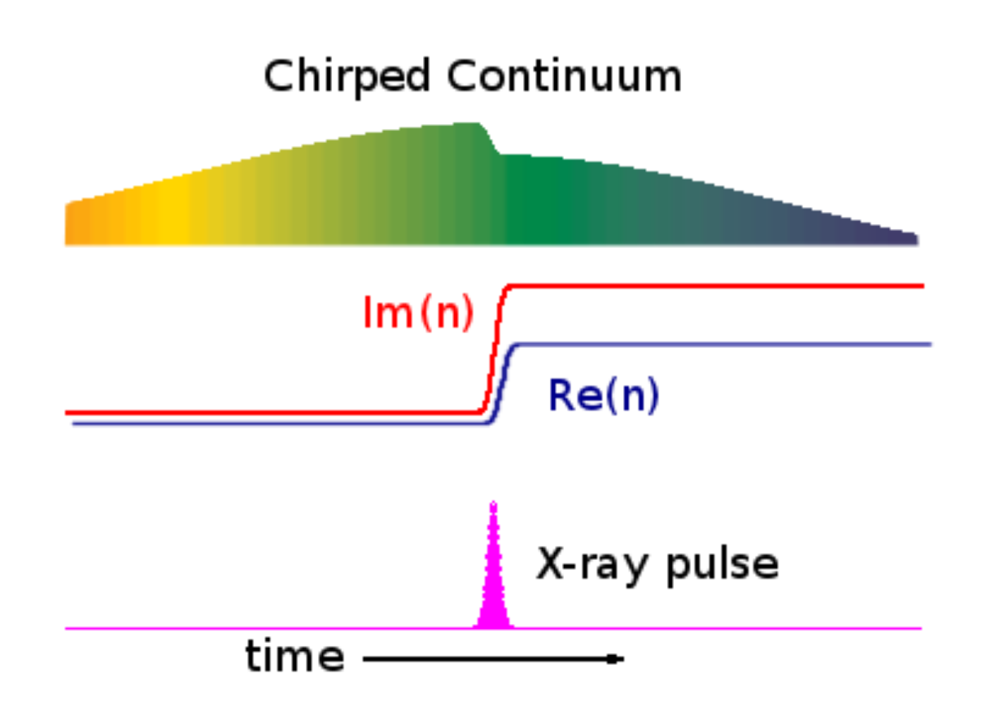
The white light propagates through the target, with shorter (bluer) wavelengths arriving first, and longer (redder) wavelengths arriving later. Somewhere in the middle of passing through the target, the x-rays join the party, hitting the target at the same place, but for a shorter temporal duration (~50 fs is typical). This causes the index of refraction of the material to change, and generates an edge in the white light power profile (in time, and therefore also spectrally, due to the chirp). See figure:
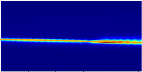
The white light, now "imprinted" with the x-ray pulse, is dispersed by a diffraction grating onto a camera. Here's what the raw signal looks like, typically:
If you take a projection of this image along the y-axis, you obtain a trace similar to this:
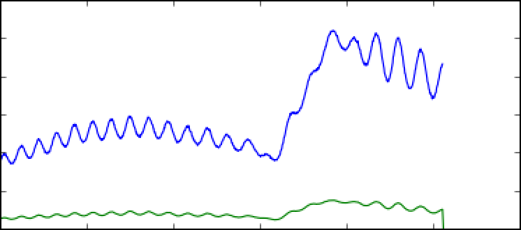
The blue line is a raw projection, the green is an ROI'd projection (recommended!). A few things to notice:
- Boom! An edge! The edge moves back and forth on the camera screen depending on the relative time delay between the laser and x-rays.
- Wiggles. The nearly-constant sine-like wave is undesirable background due to an etalon effect inside the TT target. Good analysis will remove it (read on). The etalon is especially bad here – it's amplitude and frequency will depend on the target.
- Limited dynamic range. The edge is big with respect to the camera. The TT has about ~1 ps of dynamic range in a given physical setup. That's fine, because the typical jitter in arrival times between x-rays and laser at LCLS is much less than that. Also, the white light pulse is only ~1 ps long! To change the delay "window" the TT is looking at, a delay stage is used to move the white light in time to keep it matched to the x-rays. It is important, however, to keep an eye on the TT signal and make sure it doesn't drift off the camera!
- Read right-to-left. In this image, the white light arriving before the x-rays is to the right, and following it in time takes us to the left. So time is right to left. Just keeping you on your toes.
| Info | ||
|---|---|---|
| ||
One confusing aspect for new users of the timetool is that there are a lot of laser pulses to keep track of. For any timetool setup, there will be at least three:
The first two are generated in the hutch (or nearby) by the same laser process. That means that there is a fixed, known time delay between the two. Also, that delay can be controlled using a delay stage. The timetool strategy is as follows. Imagine we start with all three pulses overlapped in time (up to some unknown jitter). Then, we set the femtosecond laser trigger to the desired delay – for instance, say, 2 ps before the arrival of the x-rays. The white light will also now arrive 2 ps before the x-rays. So we drive the delay stage (which is on the white light branch only) to move the white light 2 ps earlier. Now, the white light is overlapped with the x-rays once more! Further, we know the time difference between the fs laser and white light is exactly 2 ps. The white light can now be used as part of the timetool, as described. Measuring the jitter in delay between it and the x-rays will also give us the jitter between the fs laser and x-rays, even though the latter two are not temporally overlapped. The jitter problem is inherent in such a large machine as the LCLS. The x-ray pulse is generated waaay upstream (starting ~1 km away) and so, despite the best efforts of the laser guys, they will probably never be able to perfectly time their lasers – which originate in the hutches – to the LCLS pulse. So instead we use the timetool. |
Default Analysis: DAQ
Timetool results can be computed by the DAQ while data is being recorded and written directly into the .xtc files. This is almost always done. The DAQ's processing algorithm is quite good, and most users can employ those results without modification. This section will detail how the DAQ's algorithm works, access those results, assess their quality. Even if you are going to eventually implement your own solution, understanding how this analysis works will be useful. Further, in almost all cases, the DAQ results are good enough for online monitoring of the experiment.
How it works
The goal is to find the edge position, the imprint of the x-rays on the white light pulse, along the x-axis of the OPAL camera. To do this, the DAQ uses a matched filter – that means the filter looks just like the expected signal (an edge) and is "translated" across the signal, looking for the x-position of maximal matchy match. More technically: the filter is convoluted with the signal, and the convolution has a peak. That peak is identified as the edge "position" and gives your time signal. Here is an example of a TT trace (top) and the resulting convolution (bottom) used to locate the edge:
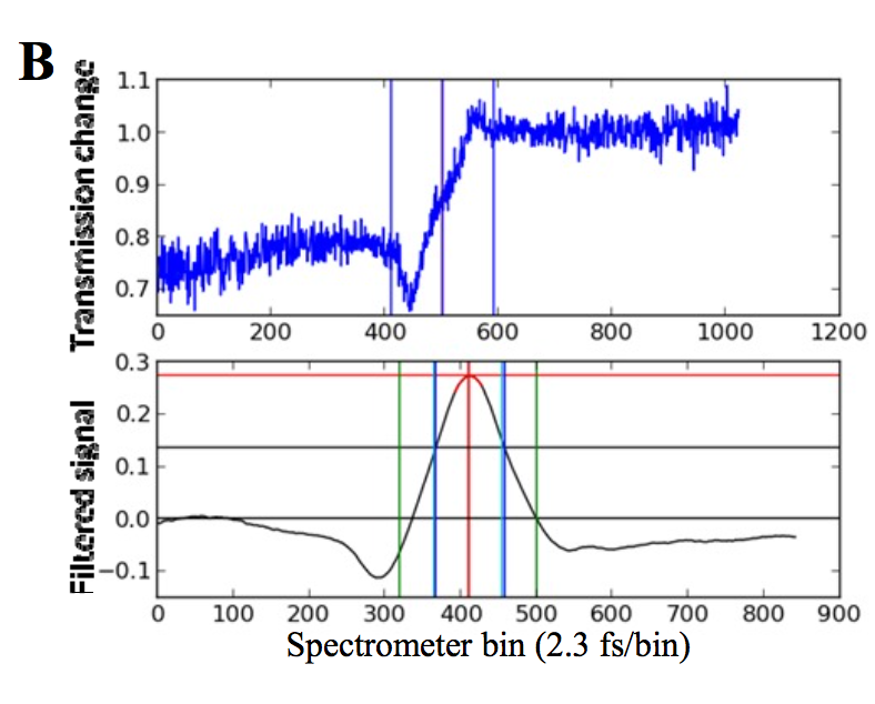
The FWHM of the convolution and it's amplitude are good indicators of how well this worked, and are also reported.
| Info | ||
|---|---|---|
| ||
| From Matt Weaver 8/23/17: (including extra thoughts transcribed by cpo from Matt on 02/26/20) The spectrum ratio is treated as a waveform, and that waveform is analyzed with a Wiener filter in the "time" domain. It is actually a matched filter where the noise is characterized by taking the ratio of non-exposed spectra from different images - should be flat but the instability of the reference optical spectrum causes it to have correlated movements. So, the procedure for producing those matched filter weights goes like this:
There's a script (https://github.com/lcls-psana/TimeTool/blob/master/data/timetool_setup.py) which shows the last steps of the calibration process that produces the matched filter weights from the autocorrelation function and the signal waveform. That script has the auto-correlation function and averaged-signal hard-coded into it, but it shows the procedure. It requires some manual intervention to get a sensible answer, since there are often undesirable features in the signal that the algorithm picks up and tries to optimize towards. The fundamental formula in that script is weights=scipy.linalg.inv(scipy.linalg.toeplitz(acf))*(averaged_signal). The above procedure optimizes the filter to reject the background. Matt doesn't currently remember a physical picture of why the "toeplitz" formula optimizes the weights to reject background. If one wants to simplify by ignoring the background suppression optimization, the "average signal" (ignoring the background) can also be used as a set of weights for np.convolve. |
The astute reader will notice that this trace has no etalon wiggles. That is because it has been cleaned up by subtracting an x-ray off shot (BYKICK). Those events have the same etalon effect, but no edge – subtracting them removes the etalon. That's a good thing, because the etalon wiggles would have given this method a little trouble if they were big in amplitude.
So, to summarize, here is what the DAQ analysis code does:
- Extract the TT trace using an ROI + projection
- Subtract the most recent x-ray off (BYKICK) trace
- Convolve the trace with a filter
- Report the position, amplitude, FWHM of the resulting peak
The reported position will be in PIXELS. That is not so useful! To convert to femtoseconds, we need to calibrate the TT.
| Info | ||
|---|---|---|
| ||
The timetool only gives you a small correction to the laser-xray delay. The "nominal" delay is set by the laser, which is phase locked to the x-rays. The timetool measures jitter around that nominal delay. So you should compute the final delay as: delay = nominal_delay + timetool_correction Since different people have different conventions about the sign that corresponds to "pump early" vs. "pump late" you must exercise caution that you are doing the right thing here. Ensure that things are what you think they are. If possible, figure this out before your experiment begins, or early in running, and write it down. Force everyone to use the same conventions. Especially if you are on night shift :). The "nominal delay" should be easily accessible as a PV. Unfortunately, it will vary hutch-to-hutch. Sorry. Ask your beamline scientist or PCDS PoC for help. |
How to get the results
Results can be accessed using the following epics-variables names:
| TTSPEC:FLTPOS | the position of the edge, in pixels |
| TTSPEC:AMPL | amplitude of biggest edge found by the filter |
| TTSPEC:FLTPOSFWHM | the FWHM of the edge, in pixels |
| TTSPEC:AMPLNXT | amplitude of second-biggest edge found by the filter, good for rejecting bad fits |
| TTSPEC:REFAMPL | amplitude of the background "reference" which is subtracted before running the filter algorithm, good for rejecting bad fits |
| TTSPEC:FLTPOS_PS | the position of the edge, in picoseconds, but requires correct calibration constants be put in the DAQ when data is acquired. Few people do this. So be wary. |
These are usually pre-pended by the hutch, so e.g. at XPP they will be "XPP:TTSPEC:FLTPOS". The TT camera (an OPAL) should also be in the datastream.
Here is an example of how to get these values from psana
| Code Block | ||||||||
|---|---|---|---|---|---|---|---|---|
| ||||||||
import psana

ds = psana.MPIDataSource('exp=cxij8816:run=221')

evr       = psana.Detector('NoDetector.0:Evr.0')
tt_camera = psana.Detector('Timetool')
tt_pos    = psana.Detector('CXI:TTSPEC:FLTPOS')
tt_amp    = psana.Detector('CXI:TTSPEC:AMPL')
tt_fwhm   = psana.Detector('CXI:TTSPEC:FLTPOSFWHM')

for i,evt in enumerate(ds.events()):
    tt_img = tt_camera.raw(evt)
# <...> |
How to know it did the right thing
Cool! OK, so how do you now if it worked? Here are a number of things to check:
- Plot some TT traces with the edge position on top of them, and make sure the edge found is reasonable.
- Look at a "jitter histogram", that is the distribution of edge positions found, for a set time delay. The distribution should be approximately Gaussian. Not perfectly. But it should not be multi-modal.
- Do pairwise correlation plots between TTSPEC:FLTPOS / TTSPEC:AMPL / TTSPEC:FLTPOSFWHM, and ensure that you don't see anything "weird". They should form nice blobs – maybe not perfectly Gaussian, but without big outliers, periodic behavior, or "streaks".
- Analyze a calibration run, where you change the delay in a known fashion, and make sure your analysis matches that known delay (see next section).
- The gold standard: do your full data analysis and look for weirdness. Physics can be quite sensitive to issues! But it can often be difficult to trouble shoot this way, as many things could have caused your experiment to screw up.
Outliers in the timetool analysis are common, and most people typically throw away shots that fall outside obvious "safe" regions. That is totally normal, and typically will not skew your results.
| Tip | ||
|---|---|---|
| ||
If you make a plot of the measured timetool delay it is quite noisy (e.g. the laser delay vs. the measured filter position, TTSPEC:FLTPOS, while keeping the TT stage stationary). There are many outliers. This can be greatly cleaned up by filtering based on the TT peak. I (TJ, <tjlane@slac.stanford.edu>) have found the following "vetos" on the data to work well, though they are quite conservative (throw away a decent amount of data). That said they should greatly clean up the TT response and has let me proceed in a "blind" fashion: Require: tt_amp [TTSPEC:AMPL] > 0.05 AND 50.0 < tt_fwhm [TTSPEC:FLTPOSFWHM]< 300.0 This was selected based on one experiment (cxii2415, run 65) and cross-validated against another (cxij8816, run 69). |
Always Calibrate! Why and How.
As previously mentioned, the timetool trace edge is found and reported in pixels along the OPAL camera (e.g. arbitrary spatial units), and must be converted into a time delay (in femtoseconds). Because the TT response is a function of geometry, and that geometry can change even during an experiment due to thermal expansion, changing laser alignment, different TT targets, etc, frequent calibration is recommended. A good baseline recommendation is to do it once per shift, and then again if something affecting the TT changes.
To calibrate, we change the laser delay (which affects the white light) while keeping the delay stage for the TT constant. This causes the edge to transverse the camera, going from one end to the other, as the white light delay changes due to the changing propagation length. Because we know the speed of light, we can figure out what the change in time delay was, and use that known value to calibrate how much the edge moves (in pixels) for a given time delay change.
Two practicalities to remember:
- There is inherent jitter in the arrival time between x-rays and laser (remember, this is why we need the TT!). So to do this calibration we have to average out this jitter across many shots. The jitter is typically roughly Gaussian, so this works.
- The delay-to-edge conversion is not generally perfectly linear. In common use at LCLS is a 2nd order polynomial fit (phenomenological) which seems to work great.
Here's a typical calibration result from CXI, with vetos applied:
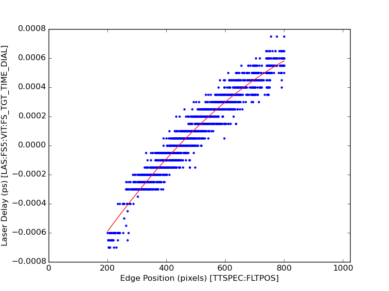
FIT RESULTS
fs_result = a + b*x + c*x^2,  x is edge position
------------------------------------------------
a = -0.001196897053
b = 0.000003302866
c = -0.000000001349
------------------------------------------------
fit range (tt pixels): 200 <> 800
time range (fs):       -0.000590 <> 0.000582
------------------------------------------------
Unfortunately, right now CXI, XPP, and AMO have different methods for doing this calibration. Talk to your beamline scientist about how to do it and process the results.
Conversion from FLTPOS pixels into ps
Once you do this calibration, it should be possible to write a simple function to give you the corrected delay between x-rays and optical laser. For example, the following code snip was used for an experiment at CXI. NOTE THIS MAY CHANGE GIVEN YOUR HUTCH AND CONVENTIONS. But it should be a good starting point ![]() .
.
| Code Block | ||||
|---|---|---|---|---|
| ||||
def relative_time(edge_position):
    """
    Translate edge position into fs (for cxij8816)

    from docs >> fs_result = a + b*x + c*x^2, x is edge position
    """
    a = -0.0013584927458976459
    b =  3.1264188429430901e-06
    c = -1.1172611228659911e-09
    x = tt_pos(evt)
    tt_correction = a + b*x + c*x**2
    time_delay = las_stg(evt)
return -1000*(time_delay + tt_correction) |
Rolling Your Own
Hopefully you now understand how the timetool works, how the DAQ analysis works, and how to access and validate those results. If your DAQ results look unacceptable for some reason, you can try to re-process the timetool signal. If, right now, you are thinking "I need to do that!", you have a general idea of how to go about it. If you need further help, get in touch with the LCLS data analysis group. In general we'd be curious to hear about situations where the DAQ processing does not work and needs improvement.
There are currently two resources you can employ to get going:
- It is possible to re-run the DAQ algorithm offline in psana, with e.g. different filter weights or other settings. This is documented extensively.
- There is some experimental python code for use in situations where the etalon signal is very strong and screws up the analysis. It also simply re-implements a version of the DAQ analysis in python, rather than C++, which may be easier to customize. This is under active development and should be considered use-at-your-own-risk. Get in touch with TJ Lane <tjlane@slac.stanford.edu> if you think this would be useful for you.
References
https://opg.optica.org/oe/fulltext.cfm?uri=oe-19-22-21855&id=223755
https://www.nature.com/articles/nphoton.2013.11
https://opg.optica.org/oe/fulltext.cfm?uri=oe-28-16-23545&id=433772a module that calculates the reference autocorrelation function from events without FEL for use in the digital filter construction.
Overview
Content Tools