...
Comparison
...
of
...
gtdiffrsp
...
output
...
with
...
gtsrcmaps
...
values
...
- The
...
- diffuse
...
- response
...
- quantities
...
- are
...
- proportional,
...
- up
...
- to
...
- an
...
- energy-dependent
...
- factor
Wiki Markup {latex}$s(E)${latex}
...
(i.e.,
...
- the
...
- spectrum),
...
- to
...
- the
...
- probability
...
- densities
...
- of
...
- a
...
- given
...
- event
...
- for
...
- the
...
- corresponding
...
- source
...
- models.
...
- If
Wiki Markup {latex}$\tilde{S}(\hat{p})${latex}
...
is
...
- the
...
- spatial
...
- distribution
...
- of
...
- the
...
- diffuse
...
- component,
...
- then
...
- the
...
- diffuse
...
- response
...
- is
Wiki Markup {latex} \newcommand{\phat}{{\hat{p}}} \newcommand{\phatp}{{\hat{p}^\prime}} \newcommand{\E}{{\epsilon}} \newcommand{\Ep}{{\E^\prime}} \begin{eqnarray} d_0(\Ep, \phatp) &= &\int d\phat \tilde{S}(\phat) P(\phatp; \E, \phat, t) A(E, \phat, t) D(\Ep; \E, \phat, t)\\ &= &\int d\phat \tilde{S}(\phat) P(\phatp; \Ep, \phat, t) A(\Ep, \phat, t) \end{eqnarray} Here, $\phat$ and $\E$ are true photon direction and energy, $t$ is the arrival time, primes indicate measured quantities, $P$ is the PSF, $A$ is the effective area, and $D$ is the energy dispersion (taken to be a delta function in energy in the second line). {latex}
...
- In
...
- gtsrcmaps
...
- the
...
- spatial
...
- distribution
...
- is
...
- multiplied
...
- by
...
- the
...
- time-integrated
...
- exposure,
...
Wiki Markup {latex}$E${latex}
...
and
...
- convolved
...
- with
...
- the
...
- mean
...
- PSF,
...
Wiki Markup {latex}$P_{\rm avg}${latex}
...
:Wiki Markup {latex} \newcommand{\phat}{{\hat{p}}} \newcommand{\phatp}{{\hat{p}^\prime}} \newcommand{\E}{{\epsilon}} \newcommand{\Ep}{{\E^\prime}} \begin{eqnarray} E(\Ep, \phat) &=& \int dt A(\Ep, \phat, t)\\ P_{\rm avg}(\phatp; \Ep, \phat) &=& \frac{1}{E(\Ep, \phat)} \int dt A(\Ep, \phat, t) P(\phatp; \Ep, \phat, t)\\ d_1(\Ep, \phatp) &=& \int_{\Delta\phatp} d\phatp \int d\phat E(\Ep, \phat) P_{\rm avg}(\phatp; \Ep, \phat) \tilde{S}(\phat) \end{eqnarray} The integral over $\phatp$ is over the pixel size, $\Delta\phatp$. For an inertial pointing, $E$ is just the effective area times the livetime $\Delta t$ and we should have \begin{equation} d_0 = \frac{d_1}{\Delta t \Delta \phatp} \end{equation} {latex}
...
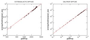
The
...
- lhs
...
- of
...
- the
...
- above
...
- equation
...
- is
...
- plotted
...
- vs
...
- the
...
- rhs
...
- below
...
- for
...
- extragalactic
...
- (isotropic)
...
- and
...
- gll_iem_v02.fit
...
- diffuse
...
- models.
...
- The
...
- red
...
- curves
...
- are
...
- best
...
- fit
...
- power-laws
...
- with
...
- the
...
- index
...
- fixed
...
- to
...
- unity.
...
- Other
...
- than
...
- a
...
- constant
...
- factor
...
- of
...
- approximately
...
- 2
...
- in
...
- both
...
- plots
...
- (2.04
...
- and
...
- 1.95,
...
- respectively),
...
- the
...
- relation
...
- holds
...
- fairly
...
- well.
...
- Replacing
...
- the
...
- gtdiffrsp
...
- values
...
- in
...
- the
...
- FT1
...
- file
...
- with
...
- the
...
- gtsrcmaps
...
- values
...
- does
...
- not
...
- result
...
- in
...
- a
...
- substantial
...
- change
...
- in
...
- the
...
- fit
...
- of
...
- the
...
- two
...
- components.
...
Npred Tests
I have run a number of 1-day simulations (idealized rocking) using Galactic (gll_iem_v02.fit)
...
and
...
extragalactic
...
(isotropic,
...
index=-2.1,
...
EGRET
...
>100
...
MeV
...
flux)
...
diffuse
...
components,
...
and
...
made
...
nominal
...
selections
...
at
...
the
...
Galactic
...
anticenter
...
(0.1-100
...
GeV;
...
ra,
...
dec,
...
rad
...
=
...
86.4,
...
28.9,
...
15).
...
For
...
each
...
realization,
...
I
...
fit
...
the
...
two
...
components
...
using
...
unbinned
...
likelihood,
...
compute
...
Npred
...
from
...
the
...
fit
...
and
...
determine
...
Nobs
...
(the
...
observed
...
number
...
of
...
events
...
with
...
the
...
ROI)
...
for
...
each
...
component.
...
In
...
order
...
to
...
search
...
for
...
biases,
...
I
...
compare
...
the
...
distributions
...
of
...
Npred
...
and
...
Nobs
...
to
...
the
...
Npred
...
values
...
that
...
are
...
obtained
...
using
...
the
...
MC
...
values
...
for
...
the
...
normalization
...
and
...
spectral
...
parameters
...
of
...
the
...
two
...
components.
...
The
...
Npred
...
values
...
using
...
the
...
MC
...
parameters
...
are
...
Npred(GalProp)
...
=
...
118.864
...
and
...
Npred(EG
...
Diffuse)
...
=
...
18.726.
...
These
...
are
...
plotted
...
as
...
the
...
dashed
...
vertical
...
and
...
horizontal
...
lines
...
in
...
the
...
figures.
...
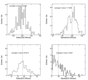
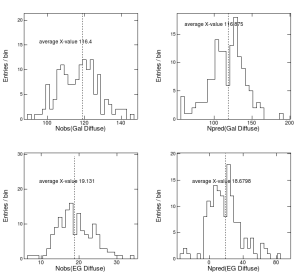
- Histograms
...
- of
...
- Npred
...
- and
...
- Nobs.
...
- Mean
...
- values
...
- of
...
- the
...
- distributions
...
- are
...
- given
...
- as
...
- the
...
- "average
...
- X-value".
...
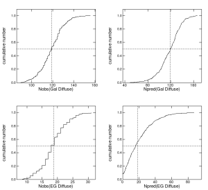
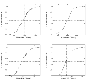
- Normalized cumulative distributions. The horizontal lines at 0.5
...
- indicate
...
- the
...
- median
...
- values
...
- on
...
- the
...
- distributions.
...
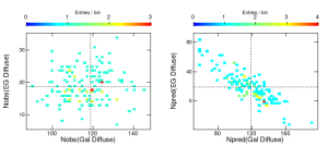
- 2D distributions.
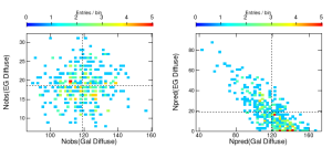
Relaxing Npred(EG Diffuse) > 0 constraint
These are the same plots, but in the fitting, the normalization of the extragalactic diffuse emission was allowed to go negative. A positive lower limit was placed on the Galactic component normalization to help prevent negative overall probability densities, but some cases (4 out of 149) still arose in the process of the optimization. These were omitted from the distributions and probably lie in the negative Npred(EG Diffuse) range, so these results are slightly biased.
- Histograms of Npred and Nobs. Mean values of the distributions are given as the "average X-value".
- Normalized cumulative distributions. The horizontal lines at 0.5 indicate the median values on the distributions.
- 2D distributions.