Content
Data sample for test
xcs01116-r0144 event 10
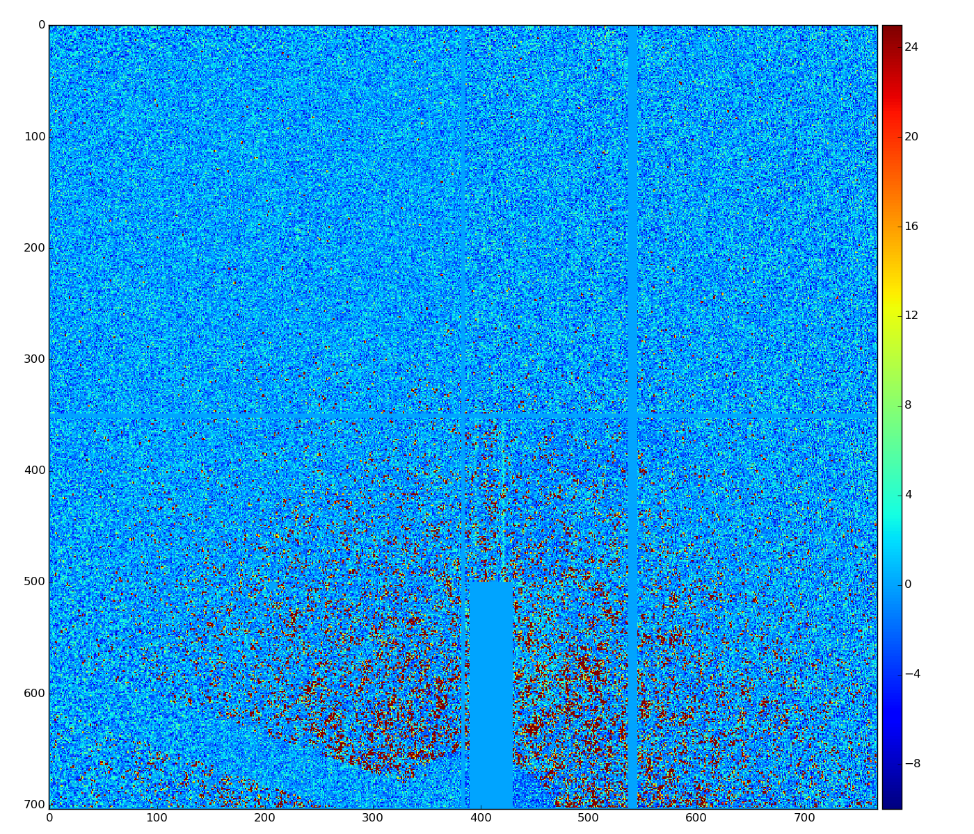
Data with subtracted pedestals
ped = det.pedestals(run)
data_ped = det.raw(evt)-ped
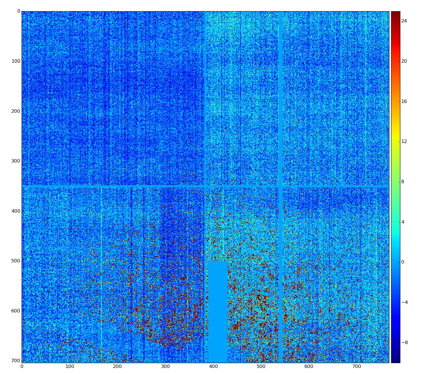
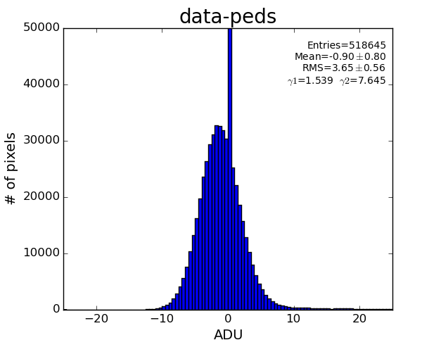
This data has structure which can be corrected.
Old version of algorithm
EPIX100A has an option to turn on up to 3 regions for common mode correction, controlled by the bitword parameter #2:
- bit#1 - common mode for 352x96-pixel 16 banks,
- bit#2 - common mode for 96-pixel rows in 16 banks,
- bit#3 - common mode for 352-pixel columns in 16 banks
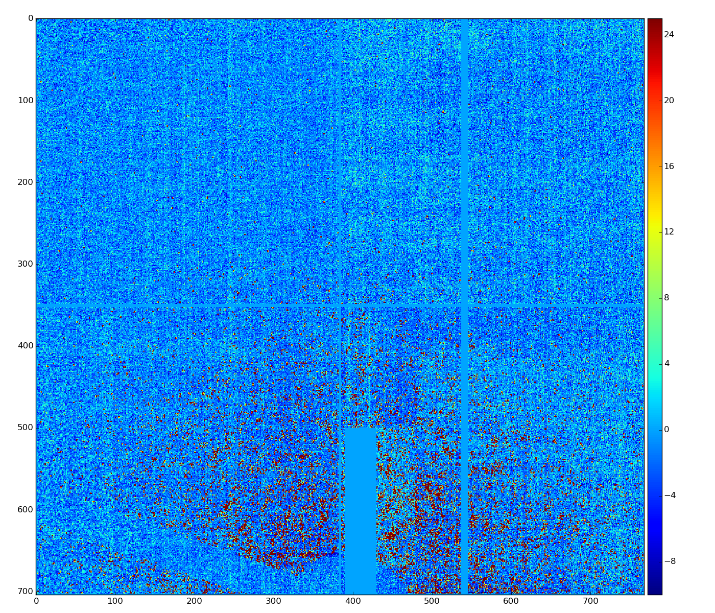
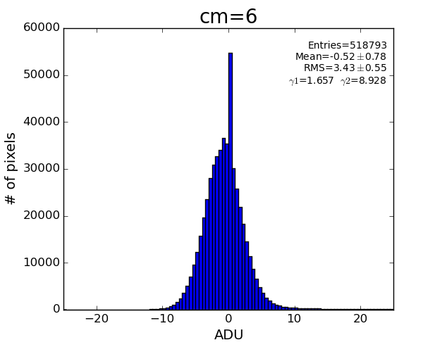
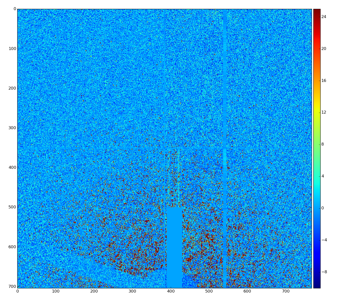
det.common_mode_apply(run, data_calib6, cmpars=(4,6,30,10))
New development
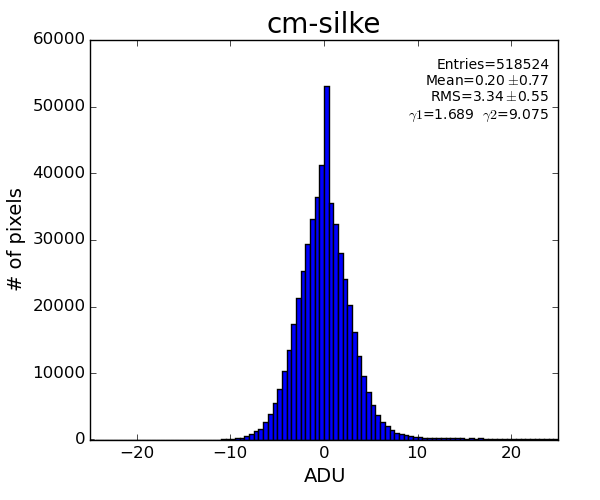
Silke Nelson has implemented similar algorithm in python, which visually demonstrates better performance
Implementation in ImgAlgos
Apparently the difference is that np.median() method in python returns median as a float value. In our old version median is integer - histogram bin number associated with integer ADU which is closest to the half histogram statistics.
A few algorithms with float common mode correction were tested and show about the same results
- meanInRegion - evaluates mean value in the range of intensities (-30,30),
- medianInRegionV2 - improved hisotgram-based algorithm; float correction to integer median position using histogram bins as weights,
- medianInRegionV3 - classic median algorithm for input array of data - this is set for production version.

det.common_mode_apply(run, data_calib6, cmpars=(4,6,30,10))
This algorithm reproduces result of Silke.
Check for other options of common mode algorithm
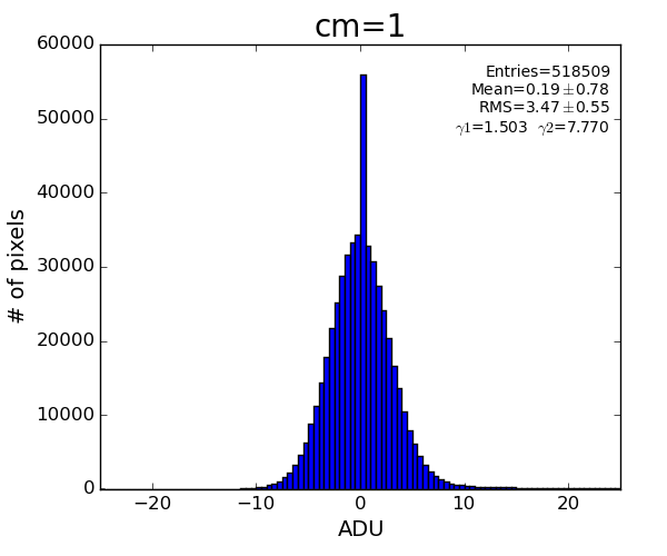
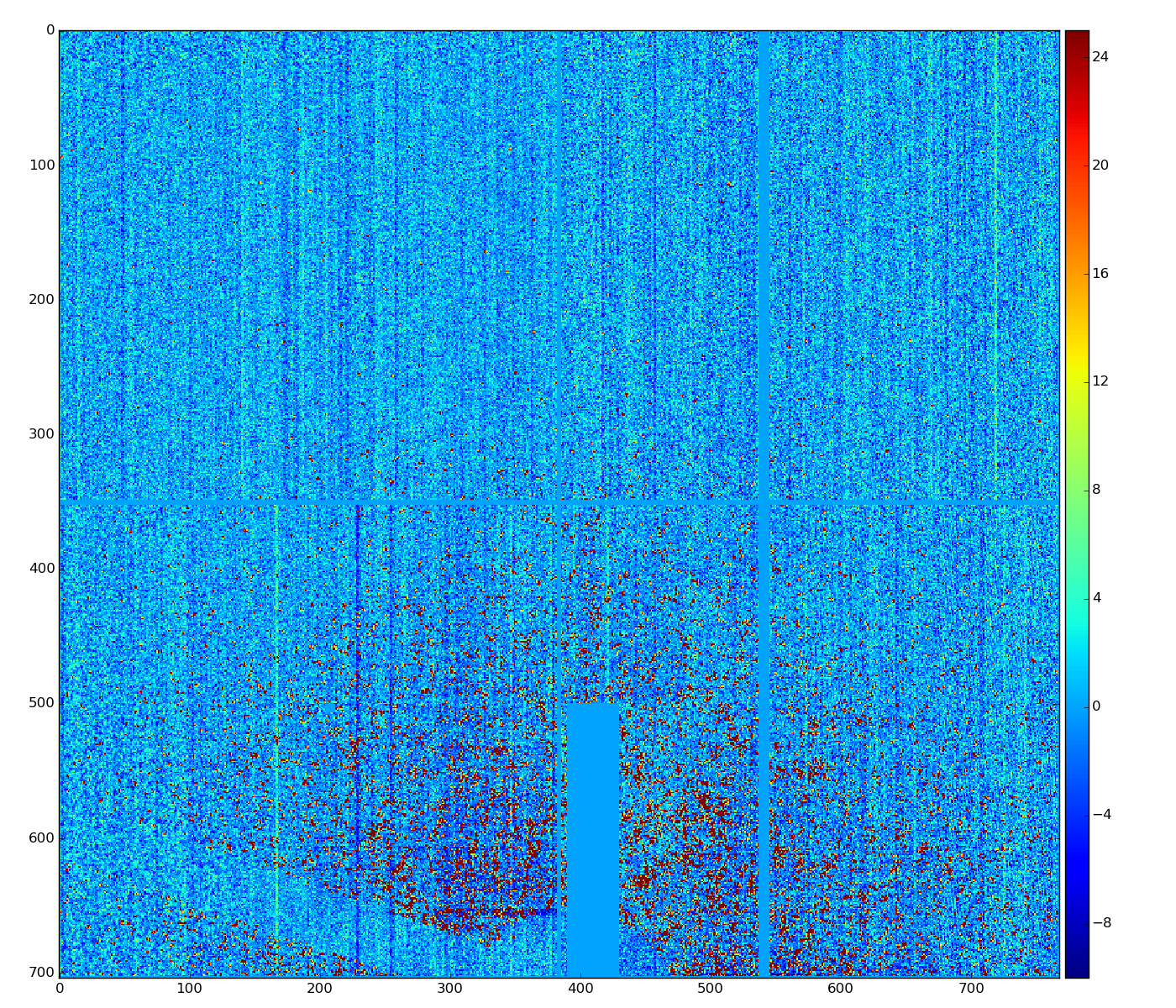
cmpars=(4,1,30,10)
bit#1 - common mode for 352x96-pixel 16 banks
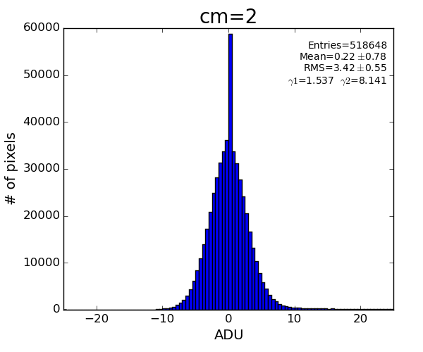
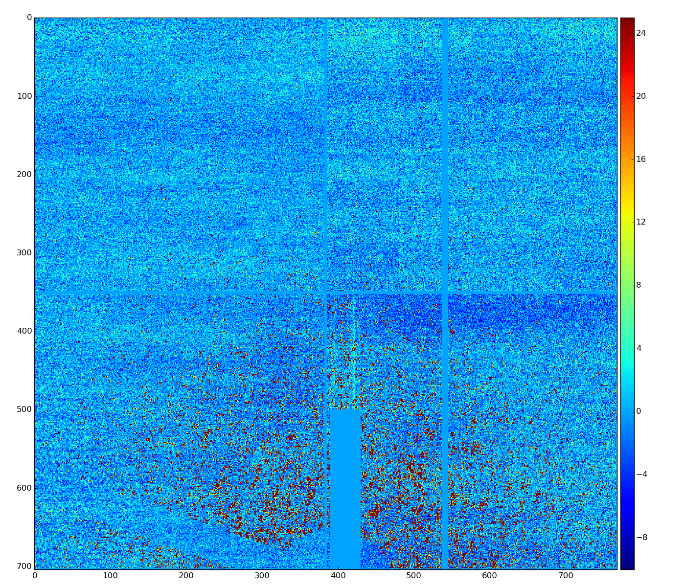
cmpars=(4,2,30,10)
bit#2 - common mode for 96-pixel rows in 16 banks
cmpars=(4,4,30,10)
bit#3 - common mode for 352-pixel columns in 16 banks

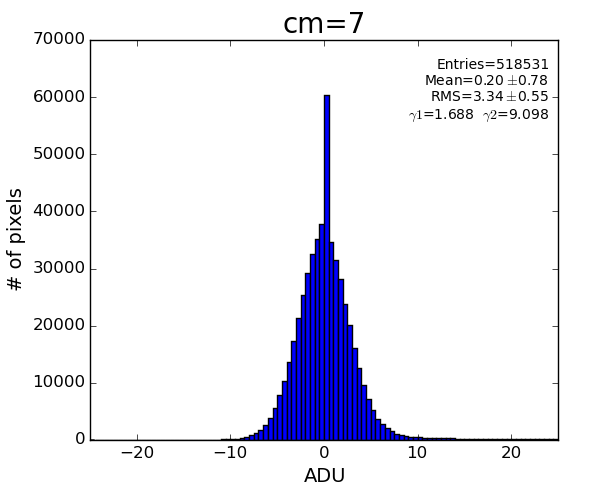
cmpars=(4,7,30,10)
combination of all three corrections

Summary
Sufficient common mode correction can be acheived with parameters cmpars=(4,6,30,10)
References
Comparison of Algorithm #4 with Algorithm #6
These two common mode algorithms were compared for exp=xcs06016:run=37 with the default parameters. The plot is shown below. Algorithm #4 has a mean of 141.535 ± 0.067 with a sigma of 8.754 while algorithm #6 has a mean of 142.153 ± 0.067 with a sigma 8.773.
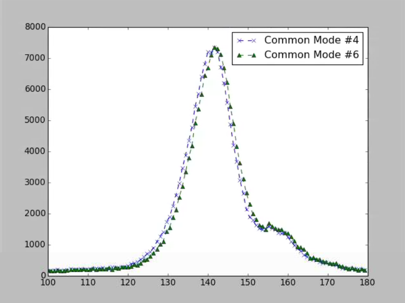
The code used to produce this plot is shown below.
from psana import *
from ImgAlgos.PyAlgos import PyAlgos
import matplotlib.pyplot as plt
import numpy as np

ds = DataSource('exp=xcs06016:run=37:smd')
det = Detector('epix_2')

tl, th = 10, 30
r, r0, dr = 1, 3.3, 0
alg4, alg6 = PyAlgos(), PyAlgos()
all_44, all_46 = np.array([]), np.array([])

for nevent, evt in enumerate(ds.events()):
    if nevent == 10: break

    nda6 = det.calib(evt, cmpars = [6], rms = det.rms(evt))
    nda4 = det.calib(evt)

    peaks_v44 = alg4.peak_finder_v4r2(nda4, thr_low=tl, thr_high=th,
                                      rank=r, r0=r0, dr=dr)
    all_44 = np.append(all_44, peaks_v44)

    peaks_v46 = alg6.peak_finder_v4r2(nda6, thr_low=tl, thr_high=th,
                                      rank=r, r0=r0, dr=dr)
    all_46 = np.append(all_46, peaks_v46)

low_lim, hi_lim = 100, 180


## Cuts off data between low_lim and hi_lim
all_44 = all_44.reshape(-1, 17)
all_44 = all_44[(all_44[:, 5] > low_lim) & (all_44[:, 5] < hi_lim)]
all_46 = all_46.reshape(-1, 17)
all_46 = all_46[(all_46[:, 5] > low_lim) & (all_46[:, 5] < hi_lim)]


hist_44, bin_edge_44 = np.histogram(all_44[:, 5], 100)
hist_46, bin_edge_46 = np.histogram(all_46[:, 5], 100)


plt.figure()
plt.plot(bin_edge_44[:-1], hist_44, linestyle='--', marker='x',
         label='Common Mode #4')
plt.plot(bin_edge_46[:-1], hist_46, linestyle='--', marker='^',
         label='Common Mode #6')
plt.legend()
plt.xlim(low_lim, hi_lim)
plt.show()
Overview
Content Tools