Investigating transfer learning, what can we do with a fully trained ImgNet model?
The idea is to take a fully trained model, like a ImgNet winner, and re-use it for your own task. You could throw away the final logits and retrain for your classification task, or retrain a few of the top layers. Carrying out this exercise with the LCLS amo86815 xtcav machine learning data involves the following steps (worked with the small, reduced xtcav data):
- Prepare the data, vggnet takes color images, [0-255] values, small xtcav is grayscale, [0-255].
- vggnet subtracts one number from each of RGB, the mean per channel, need to calucate our mean value
Dataset
The reduced xtcav, took runs 69, 70 and 71, but for run 70 and 71, conditioned on acq.enPeaksLabel >=1 to make sure some lasing was measured. About 20,000 no-lasing samples from run 69, and 40,000 lasing samples.
Goal: Just learn lasing from no lasing - we have so much of this data, the end goal is to build good models that can be used to 'declutter' or split of signal from reference (see Project Ideas - Declutter/Discovering Science)
Preprocess
vggnet works with 224 x 224 x 3 color images. simplest way to pre-process, replicate our intensities across all three channels

Question
What is the best way to preprocess our data for a imagenet model? Is there a better way to take advantage of the encoding of our 16 bit ADU images into 24 bit RBG? idea:
- use a colormap - that is colorize as above, with blue for dark, red for bright
If we were to train from scratch, I think we should make two channels, that is channel 1, the 'red' channel, is the high 8 bits of the 16 bit ADU, and channel 2 is the low 8 bits. This would mimic red being a brighter color color.
Note
vggnet does not mean center the images, but it subtracts the per channel mean for each or R,G,B, that is it subtracts 123.68, 116.779, 103.939 repsecively from the channels. We compute this over our small xtcav dataset and get 8.46 for each.
codewords
vggnet, http://cs231n.stanford.edu/slides/winter1516_lecture7.pdf, around slide 72, after 5 convnet layers, with relu's and max pooling, produces 7 x 7 x 512 (25,088 numbers).
Then three fully connected layers, the first two are 4096, the last, the logits, 1000 for the imagenet classes. The terminology 'codeword' refers to the final fc layer (which had relu activation producing the output) before doing classificaiton with the 'logits' (ref: http://cs231n.stanford.edu/slides/winter1516_lecture9.pdf around slide 12).
If we plot 4000 of the nolasing, then 4000 of the lasing, you get the following, make sure you click, and then hit the + input to zoom, zoom in around the 4000 split to see the marked change in the codewords as we go from lasing to no lasing:
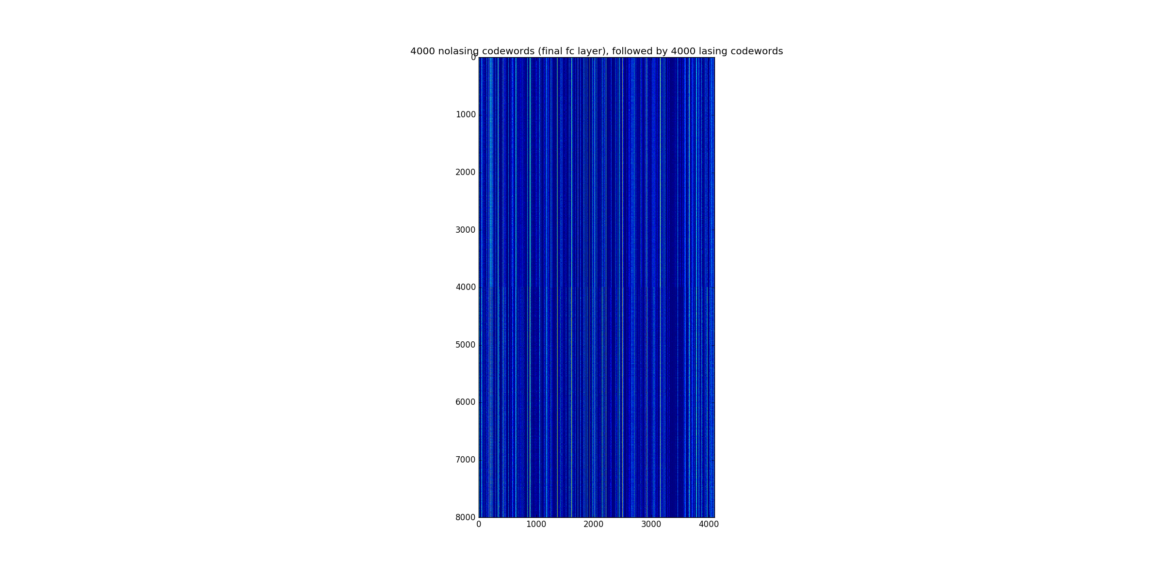
Things to note
little variation
dead neurons
still - definite difference at 4000, appears like enough to discriminate
Classifiying using Codewords
A few experiments - the mean's of the nolasing vs lasing codewords are 16.8 apart (euclidean distance).
The question is how linearly separable are the lasing/no-lasing codewords.
Classifying based on euclidean distance to the mean gives 59% accuracy.
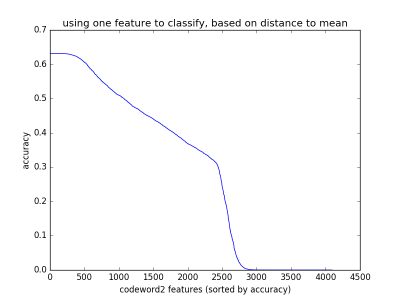
Selecting the one best feature of the 4096 components of the codeword, and classifying based on euclidean distance to the mean gives 63% accuracy. The below plot is the accuracy of each of the 4096 components, when used as a single feature, sorted by best feature. Strange why there are two elbows?
A linear classifier, trained with cross entropy loss, get 99.5%, but this is probably not the best classifier to use - I think better will be SVM based with a good margin.
Finding the Reference
We are not interested in a good classifier though, our metric is if we can find the right reference for a lasing shot, by using eclidean distance in the codeword space.
Below we take a lasing image, and find the no lasing image with the closest codeword. I looked through about 5 of these, I think they all looked similar. There is a lot of variation among lasing shots, so these images are relatively similar, but definitely not lined up horizontally.
Things to note
We could use data augmentation, to get a better match, that is for each no lasing shot, slide it around horiziontally and maybe a little vertically if need be - one of these would definitely be a better match in this case.
Ideas
You really want a codeword embedding that puts the fingers in a few separate features are orthogonal to the lasing, maybe there is a way to guide the learning to make this so?
- imagine adding a loss term that guides lasing and no-lasing codewords to have the same statistics on most of the vector, and no-lasing to be zero on a few components while lasing can use them to discriminate
I see how sparse our representation is, and I think we need PSImageNet - photon science image net - what if we took all the detector images we had, large, small, timetool, cspad, with a 1000 labels of what they are, trained a classifier. This would be a model that has learned about many nuances in our detector images, or we could combine our data with imagenet data. A better model for transfer learning?