Running an XAL Model and Upload to Oracle

This page describes the process of running an XAL model of the LCLS accelerator, and uploading that model to Oracle, from where it can be accessed by Matlab and Java applications through AIDA.

Running and Uploading the Online XAL Model

To run an XAL model, you can use the interactive matlab scripts xalRunModel.m or xalGetModel.m. These can be run directly from matlab, or from lclshome (as described below). The basic process is the same in either case - xalGetModel additionally plots dispersion, betas, and energy.

Cheatsheet - Summary of running the model using xalGetModel:
This is the basic procedure for running and uploading a model. For more details, see the sections Running a Model and Uploading a Model below.

• Select a beamline to be modelled
• Decide whether to run extant or design model
• If "extant", run LEM lite, to check energy profile
• Run the XAL model (can take 30s - 1 minute). Check resulting energy.
• [If you ran xalGetModel, then inspect the model plots ]
• Run the XAL XML Writer (to create the model upload file)
• Upload the model to the database. Password for upload is here.
  Note: there is no "back" facility. Just abort (ctrl-c to get to the matlab prompt, and start over).

Running a Model in Detail

This procedure runs through what you have to do to run a new model whose output will be used by LCLS applications. Click on any of the thumbnail images for a larger view.

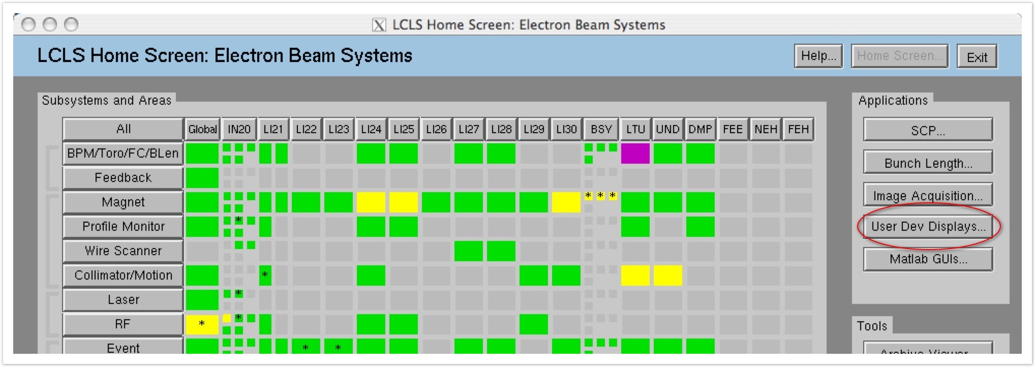
1. From lclshome, select User Dev Displays panel.  

   
   

2. Run one of the matlab scripts xalRunModel or xalGetModel
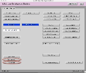
    *xalRunModel* simply runs the model and creates the upload files
    *xalGetModel* is as xalRunModel, but additionally returns ("gets") the model data to your matlab session. It also creates model plots. 
   Either of these buttons will start the corresponding matlab script...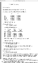
   ... which immediately prompt for you to *Select a beamline* : 
   \\
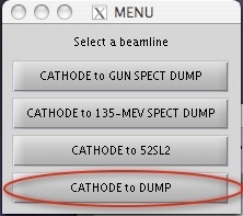   The following is a run-through of running xalGetModel for the Extant machine. [Click here to see the full transcript of this example ].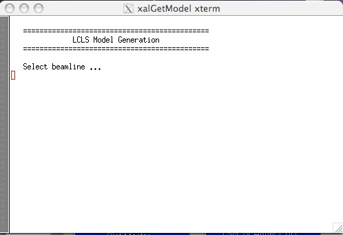   
   The procedure is as follows:

   
   

   
   

   1. For example, select "Cathode to Dump" (as shown in the example above). This runs the LCLS "Full Machine" model, from the LCLS Cathode to the main Dump. See Why are all models from Cathode to some location.

   2. *Select whether to "Run extant machine or design model? (x/d) \[d\]:*". Hit x or d, and RETURN.
       Running the "design" model (choice "d") causes the XAL model to be run with the element setpoint values in the model input files. Those design setpoint values are, [to the extent possible, identical to the MAD design|#modeldiffs]. Running the "extant" model (choice "x") will cause the model execution to first replace the design values of beamline devices, with the actual readback values, as acquired through EPICS and AIDA, prior to running the envelope tracker.  That is, "extant" is equivalent to what was called "DATABASE" in the SLC modelling system; it describes the extant machine at the time the model is run.

      *Stages of running the (extant) model are as follows:*

      
      

      • *1) "Initial Twiss"* is displayed. Check the initial conditions which will be used for the model run. These are presently taken from the SLC marker point 80. You can check these at any time with AIDAWeb ([MARK:VX80:80//twiss MODE=5|https://seal.slac.stanford.edu/aidaweb/dispatchQuery?Query=MARK%3AVX00%3A80%2F%2Ftwiss+MODE%3D5&Query+Action=Get+Data]; the values are Energy (GeV), psix, betax (m), alphax , etax (m), etax', psiy, betay (m), alphay, etay (m), etay')
        If these appear fine, then confirm to continue.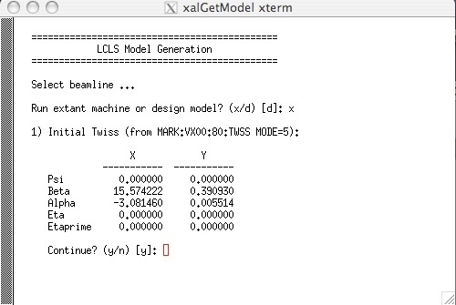

        
        

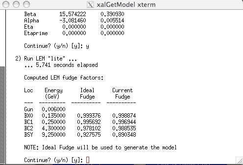
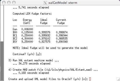
      • *2) "Run LEM 'Lite'"*. This will calculate and display the fudge factors and predicted energy. When it has completed, _check in particular that the final energy at the undulator_ (see Energy column, and the row of output labelled "BSY") is reasonable, e.g. 9.25 GeV. If energy appears fine, then confirm to continue.

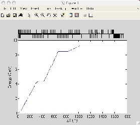
      • *3) "Run XAL machine model."* This can take up to a minute to execute, so please be patient. When it has completed, if you ran xalGetModel, you should get 3 plots - the dispersion, betas, and energy vs Z. The plots may overlap, and the energy plot is on the bottom, so move the others to check it.

        
        

        
        

        
        

      • 4) "Create MAD patch file". This stage is always entered, you don't need to do anything. It only takes a moment to create these.

      • "Create and upload XML model files to Oracle? (y/n) \[n\]: " If it all looks good, and you want to upload to Oracle, say "y".

        
        

      • 5) "Run XML writer." If you said "y" to create the upload files, you'll now see "Run XML writer." This is where the file containing the model results to be uploaded to Oracle, is created. This also takes half a minute or so.
        When it has completed, you should see that 3 files have been created: E.g.

        /u1/lcls/physics/onlinemodel/xal/xalElements_20090120_115855.xml created
        /u1/lcls/physics/onlinemodel/xal/xalDevices_20090120_115855.xml created
        /u1/lcls/physics/onlinemodel/xal/xalModel_20090120_115855.mat created
        

   3. Upload the XAL model online on the web.
      The last part of xalGetModel gives some tips of uploading. It remins you where to find the model files in the browser, and the URL of this help. See next the section of help with uploading the model files.

Uploading the XAL model files

After running the models and creating the online model output files, we must upload their data to the Oracle model server. From Oracle the data can be inspected, or retrieved through AIDA.

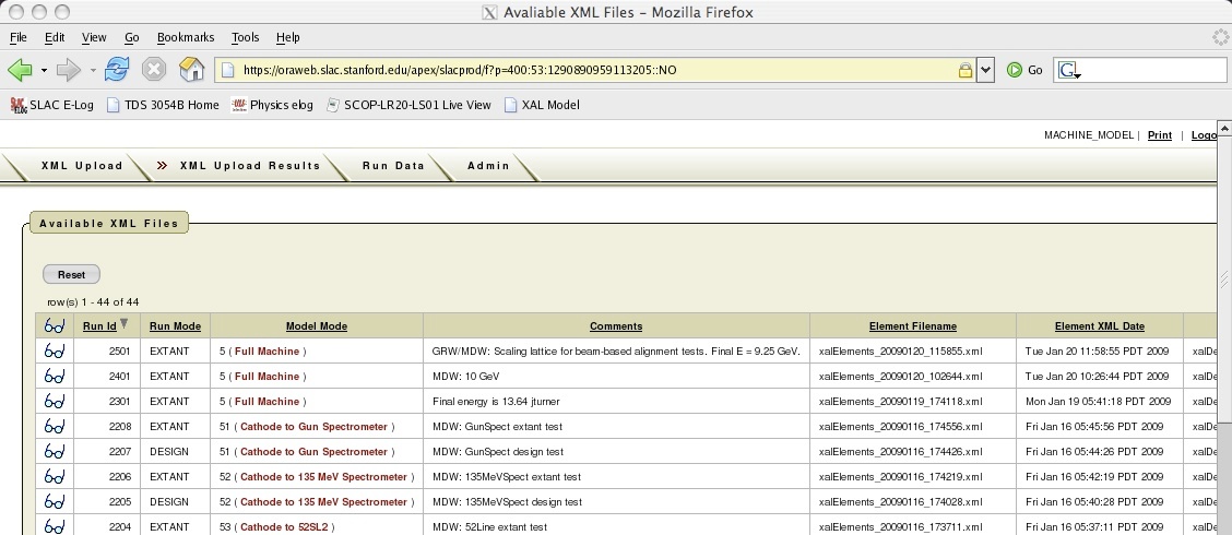
At the end of running the model, xalGetModel or xalRunModel should have launched a Firefox browser, open at the web page you use to upload the model into Oracle. The Firefox page should look like this: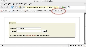

The password for user name MACHINE_MODEL, is recorded in the physics logbook entry /lclselog/data/2009/02/06.01

If you do NOT see this page (and unfortunately, sometimes Firefox does fail to start at the right page) you can use the "XAL Model" tab (see picture) in Firefox to take you to there.

You can log into the web application at any time at the URL: https://oraweb.slac.stanford.edu/apex/slacprod/f?p=400. (See note on supported hosts) You might want to do this to inspect the data

The procedure for uploading the model files into Oracle:

Once you're in the web application you should see "Select Device File" and "Select Elements File". These 2 files (of the 3) created by the above model running procedure must be uploaded to Oracle in unison. When a file has been entered for BOTH of these, you can hit "Submit" at the bottom of the dialog screen to start the process of Upload into Oracle.

1. Select Device File
   Hit the "Select Device File" button. You can either enter a full filename by hand, or use the filebrowser, to browse to /mccfs2/u1/lcls/physics/onlinemodel/xal/ and select the Devices file you created in the process above. in our example above this files was named "xalDevices_20090120_115855.xml". (Tip: since there are many files in this directory, hit "Last Modified" twice, to sort the files by date, latest first). Select the xalDevices file you created, and hit the Open icon (with a picture of a folder!) in the filebrowser dialog to make the selection. (It's a bit confusing using the word "Open" to mean "Select" - talk to Oracle about that - they went cheap and used the firefox file selection widget, designed for selecting a file to open, but they use it to mean "select").
2. Select Elements File
   Hit the "Select Elements File" button. The filebrowser should open at the right directory - amazing! Hit "Last Modified" twice to sort the files again, and click on the xalElements file you created in step 2.2.5 above. Hit "Open".
   (You do not need to upload the xalElements file at all).
3. Comments.
   Enter a comment. Please include 2 items in your comment:
   • Your name, nickname, mark, catchphrase, or other distinguishing refrain from which your personal guilt can be established.
   • The Energy at the undulator predicted in step 2.2.3 above!

4. *Submit*.
   When you are finished, the screen should look something like this: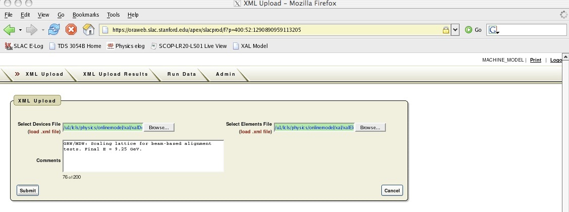

   Hit the "Submit" button. The time to upload is about 1 minute! Note that additional time is presently spent creating the screen which echos the upload data, but in fact the model data is available for use as soon as you see the XML Upload Results table:

   
   

   
   

Review the model data.

Hit the "Run Data" tab to review the uploaded results of any model which has been uploaded, including the last. Hit the little spectacles icon next to a model upload to view the model parameters of each element calculated as part of that model.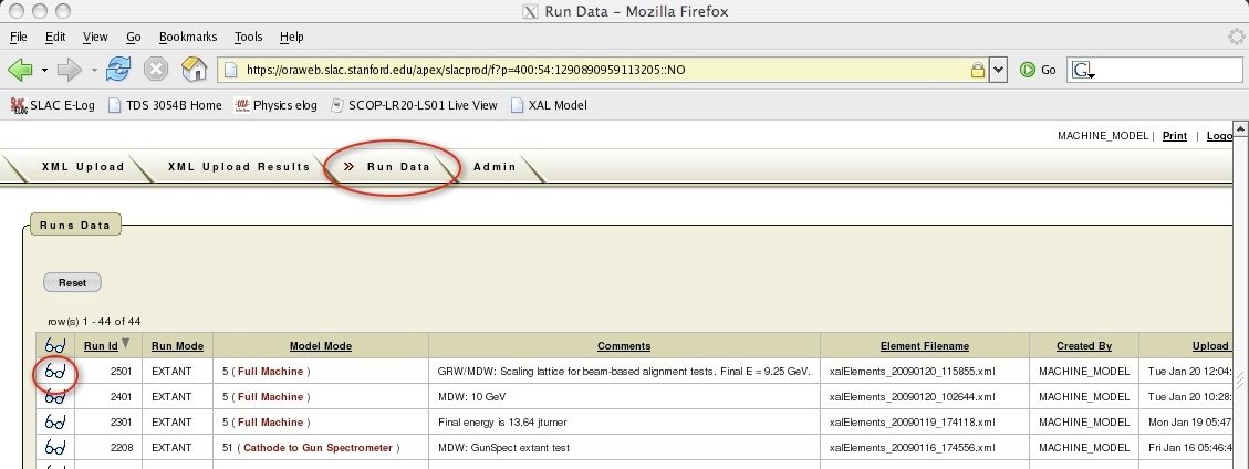

This interface takes a while to load the data, but it can do it for any uploaded model.
Alternatively, use AIDA to check the Rmats of the model elements for the latest upload.

AIDA Model Queries

Model Notes

Why are all models from Cathode to some location?

Note that all models require the model to be run from the Cathode to some beam destination, rather than allowing sections to be run independently. This is so that, for now, we can guarantee that physics computations carried out from a number of different devices throughout the machine, are carried out from consistent models made from the same initial conditions. With this technique all devices towards the photon end of the machine, must have been modeled by a model run that incorporated upstream devices. A simple example being Rmat A to B from a corrector in the injection line, to a BPM in the

Why mccfs2 in upload stage, but not in writing?

Note, the directory name starts /u1 when the files are written, but when we do the file upload from lcls-prod02 it will start /mccfs2_, that's because on lcls-prod02 the directory is accessed through an NFS server mount, which is named mccfs2.

Differences between XAL and MAD models.

To be added:
Which devices are not modelled.
What is not modelled as it is in MAD.

Update the AIDA Directory service

This section is included for completeness. It is NOT now normal to run this procedure after every model upload, since new devices are seldom added, so please don't bother! Also, Elie has written an automatic procedure to replace this, so we don't have to do it by hand.

Having uploaded a new model, we have to tell Aida to update its database of the names of XAL modelled devices. We will teach first aidadev, then aidaprod databases. These are, respectively, the Oracle usernames (ie subschema) of the Aida directory services used on the aida development and production networks.

Log into an AFS Solaris machine like tersk02, and set up the cdsoft environment

ssh -l<your-username> tersk09
tersk> source /afs/slac/g/cd/soft/dev/script/ENVS.csh

Enter sqlplus for user AIDADEV on database SLACPROD (SLACPROD will be set by sourcing ENVS.csh above).

sqlplus AIDADEV/<aidadbpassword> 

Run the updating procedure. This will look in the ELEMENT_MODELS which was updated by the APX load above, and, for every row that has a match in LCLS_ELEMENTS, it will update Aida's directory service with a name composed of the EPICS name of the device + '//twiss' and '//R', and tell Aida that that device's model is to be acquired from the XAL Aida data provider (service id 202).

aida_xal_names_update takes an optional parameter, to specify whether or not to set the service-id to 202 of names it finds to be already in the aida directory. The default (or "N") is not to set the service-id (that is, leave names which are in both the SLC namespace and EPICS name, assigned to the SLC modelling environment (service id 63). If given, and valued "Y", all names modelled by XAL will be assigned to the XAL model service id (202). That is, while we're testing XAL, use the default; when we're sure about XAL, with an EXTANT machine model, and a plan for what to do when devices for like the end station need model, then use Y to switch all modelling of those devices over to XAL.

SQL> exec aida_xal_names_update [Y];

PL/SQL procedure successfully completed.   <-- you should see this

It should tale only a few seconds.

You can see which names are assigned to the XAL model server by AIDA, use the following sql script

SQL> @show_IA_given_serviceid 202

Now go over and update the AIDAPROD names too (don't wait, all names should be in sync), run aida_all_changes again, and verify the names added again.

SQL> connect aidaprod/<aidadbpassword>
Connected.
SQL> exec aida_xal_names_update [Y];
SQL> @show_IA_given_serviceid 202

Test the upload by asking Aida to retrieve the model parameters (twiss or R) of a device in the model file uploaded. This link takes you to the AidaWeb modelling page, from where you can as for teh names of devices (eg 'BPMS:%//twiss' will return the names of all modelled BPMS, or 'BPMS:IN20:521//twiss' will return model for that device.

https://seal.slac.stanford.edu/aidaweb/modelling.jsp