...
| Metric \ Monitor Target | pinger to pinger-raspberry | pinger-raspberry to pinger | pinger to sitka | pinger-raspberry to sitka | sitka to pinger | sitka to pinger-raspberry | pinger to CERN | pinger-raspberry to CERN |
|---|---|---|---|---|---|---|---|---|
| Time period | June 17 - July 13, 2015 | June 17 - July 13, 2015 | June 17 - July 14, 2015 | June 17 - July 14 | July 15 - July 16 2015 | July 15 - July 16 2015 | June 17 - July 12, 2015 | June 17 - July 12, 2015 |
| Samples | 10890 | 10850 | 10900 | 10850 | 820 | 820 | 10900 | 10900 |
Min RTT | 0.43 ms | 0.41 ms | 22 +- 1 ms | 22.3 +- 1 ms | 22 ms | 22.4 ms | 150 +- 1 ms | 151 ms |
| Avg RTT | 0.542 +- 0.06 ms | 0.529 +- 0.5ms | 23.9 +- 1ms | 23.827 +- 1 ms | 22.30 ms | 22.709 ms | 150.307 +- 2.4 ms | 151.024 +- 1.3 ms |
Max RTT | 1.15 ms | 20.8 ms | 761 ms | 334 ms | 26.3 ms | 25.9 ms | 288 ms | 183 ms |
| Stdev | 0.055 ms | 0.540 ms | 9.58 ms | 9.60 ms | 0.219 ms | 0.222 ms | 2.37 ms | 1.3 ms |
| Median RTT | 0.542 +- 0.05 ms | 0.51 ms +- 0.052 ms | 22.3 +- 0.2 ms | 22.7 +- 0.11 ms | 22.3 +- 0.11 ms | 22.7 +- 0.21 ms | 150 +- 1 ms | 151 +- 0.01 ms |
| 25% | 0.514 ms | 0.48 ms | 22.2 ms | 22.69 ms | 22.3 ms | 22.8 ms | 149.99 ms | 150.99 ms |
| 75% | 0.564 ms | 0.532 ms | 22.4 ms | 22.8 ms | 22.19 ms | 22.59 ms | 151 ms | 151 ms |
| IQR | 0.05 ms | 0.052 ms | 0.2 ms | 0.11 ms | 0.113 ms | 0.210 ms | 1.01 ms | 0.01 ms |
| Min IPD | -0.59 ms | -20.29 ms | -244 ms | -235.1 ms | -0.4 ms | -0.39 ms | -137 ms | -32 ms |
| Avg IPD | 0 ms | 0 ms | 0 ms | 0 ms | 0 ms | 0 ms | 0 ms | 0 |
| Max IPD | 0.62 ms | 20.26 ms | 268 ms | 146 ms | 3.6 ms | 3.29 ms | 138 ms | 32 ms |
| Median IPD | 0 +- 0.07 ms | 0 +- 0.05 ms | 0 +- 0.2 ms | 0 +- 0.2ms | 0 ms +- 0.2 ms | 0 +- 0.2 ms | 0 +- 0.01 ms | 0 +- 0.01 ms |
| Stdev | 0.248 ms | 0.296 ms | ||||||
| 25% IPD | -0.04 ms | -0.03 ms | -0.1 ms | -0.11 ms | -0.1 ms | -0.1 ms | -0.01 ms | -0.01 ms |
| 75% IPD | 0.03 ms | 0.02 ms | 0.09 ms | 0.1 ms | 0.01 ms | 0.09 ms | 0 ms | 0 ms |
| IQR IPD | 0.07 ms | 0.05 ms | 0.190 +- 0.5 ms | 0.210 +- 0.4 ms | 0.2 ms | 0.190ms | 0.01 ms | 0.01 ms |
| Min(abs(IPD)) | 0 ms | 0 ms | 0 ms | 0 ms | 0 ms | 0 ms | 0 ms | 0 ms |
| Avg(abs(IPD)) | 0.041 ms | 0.066 ms | 0.424 ms | 0.406 ms | 0.120 ms | 0.139 ms | 0.386 ms | 0.046 ms |
| Max(abs(IPD)) | 0.0628ms | 20.294 ms | 268 ms | 235.1 ms | 4 ms | 3.29 ms | 138 ms | 32 ms |
| Stdev | 0.248 ms | 0.262 ms | ||||||
| Median(abs(IPD)) | 0.03ms | 0.024 ms | 0.09 ms | 0.1 ms | 0.1 ms | 0.09 ms | 0 ms | 0 ms |
| 25%(abs(IPD)) | 0.01ms | 0.008 ms | 0.01 ms | 0.01 ms | -0.01 ms | -0.01 ms | 0.01 ms | 0.01 ms |
| 75%(abs(IPD)) | 0.058 ms | 0.05 ms | 0.1 ms | 0.19 ms | 0.1 ms | 0.19 ms | 1 ms | 0 ms |
| IQR(abs(IPD) | 0.048 ms | 0.042 ms | 0.09 ms | 0.11 ms | 0.11 ms | 0.2 ms | 0.009 ms | 0.01 ms |
| Loss | 0% | 0% | 0% | 0.008% | 0% | 0% | 0% | 0% |
Since the timestamps of measurements for one MA to a target are not synchronized with another MA to the same target, they are sampling the network at different times. Thus we decided not to use the residuals in the RTTs between one pair and another. Typically the difference in the time of a measurement from say pinger.slac.stanford.edu to sitka.triumf.ca versus pinger-raspberry.slac.stanford.edu to sitka.triumf.ca averages at 8 mins (see spreadsheet mtr-localhost tab diff mtr).
To find the probability of the distributions overlapping we can use a nomogram of mean differences versus error ratios given in Overlapping Normal Distributions. John M. Linacre for normal distributions. However this does not cover the range we are interested in.
We used the Z Tests to compare two samples, see for example “Comparing distributions: Z test” available at http://homework.uoregon.edu/pub/class/es202/ztest.html
Spreadsheet (ipdv-errors) has min/avg/max, % and loss between and from pinger & pi to & from sitka, and to cern, plus histograms probabilities, IPDV errors.
Spreadsheet (prob) (Probability table as submitted, IPDV from SLAC to TRIUMF. Also images of IPD graphs from frequency.pl. The IPD distribution from pinger to SLAC has the figure below.
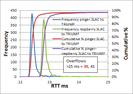
However the ping distributions are decidedly non-normal (see for example the figure below) have wide outliers, and are heavy tailed on the upper side (see https://www.slac.stanford.edu/comp/net/wan-mon/ping-hi-stat.html). This leads to large standard deviations (one to two order of magnitude greater than the IQR) in the RTT values. As can be seen from the table this results in low values of the Z-test and a false probability of no significant statistical difference. Using the IQRs of the frequency distributions instead generally leads to much higher values of the Z-test and hence a higher probability that the distributions of RTTs between two pairs of hosts are significantly different. Comparing the frequency distributions it is seen that there is indeed a marked offset in the RTT values of the peak frequencies and a resultant difference in the cumulative RTT distributions, Using the non-parametric Kolomogorov Smirnoff test (KS test) also indicated significant differences in the distributions.
Average RTTs from pinger.SLAC and pinger-raspberry.slac to TRIUMF (Figure can be found in https://confluence.slac.stanford.edu/download/attachments/192190786/ipdv-errors.xls) The plot cuts off at about the cumulative 98%. The number of overflows not plotted are indicated. |
|---|
 |
The RTT measurements made from pinger.SLAC and pinger-raspberry.SLAC to TRIUMF and CERN average around 23ms and 151ms respectively. Despite this large difference in average RTTs', comparing the average RTTs from pinger.SLAC with those from pinger-raspberry.SLAC yields a difference of only ~0.35ms for both TRIUMF and CERN.
Looking at the traceroutes, using Matt's traceroute to measure the RTT to each hop, indicates that this difference starts at the first hop and persists for later hops. See spreadsheet (MTR tab). We therefore made ping measurements from each SLAC MA to its loopback network interface. The measurements were made at the same times to facilitate comparisons. They indicate that the pinger-raspberry.SLAC is ~0.13ms lslower in responding than the pinger.SLAC MA. Thus approximately 1/3rd of the difference in average RTS tro TRIUMF measured by the two SLAC MAs is due to the MA platform itself.
IPDV
PingER's main metric for measuring jitter is the IPDV. A typical IPD distribution from which the IPD is derived is shown below.
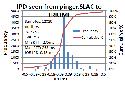
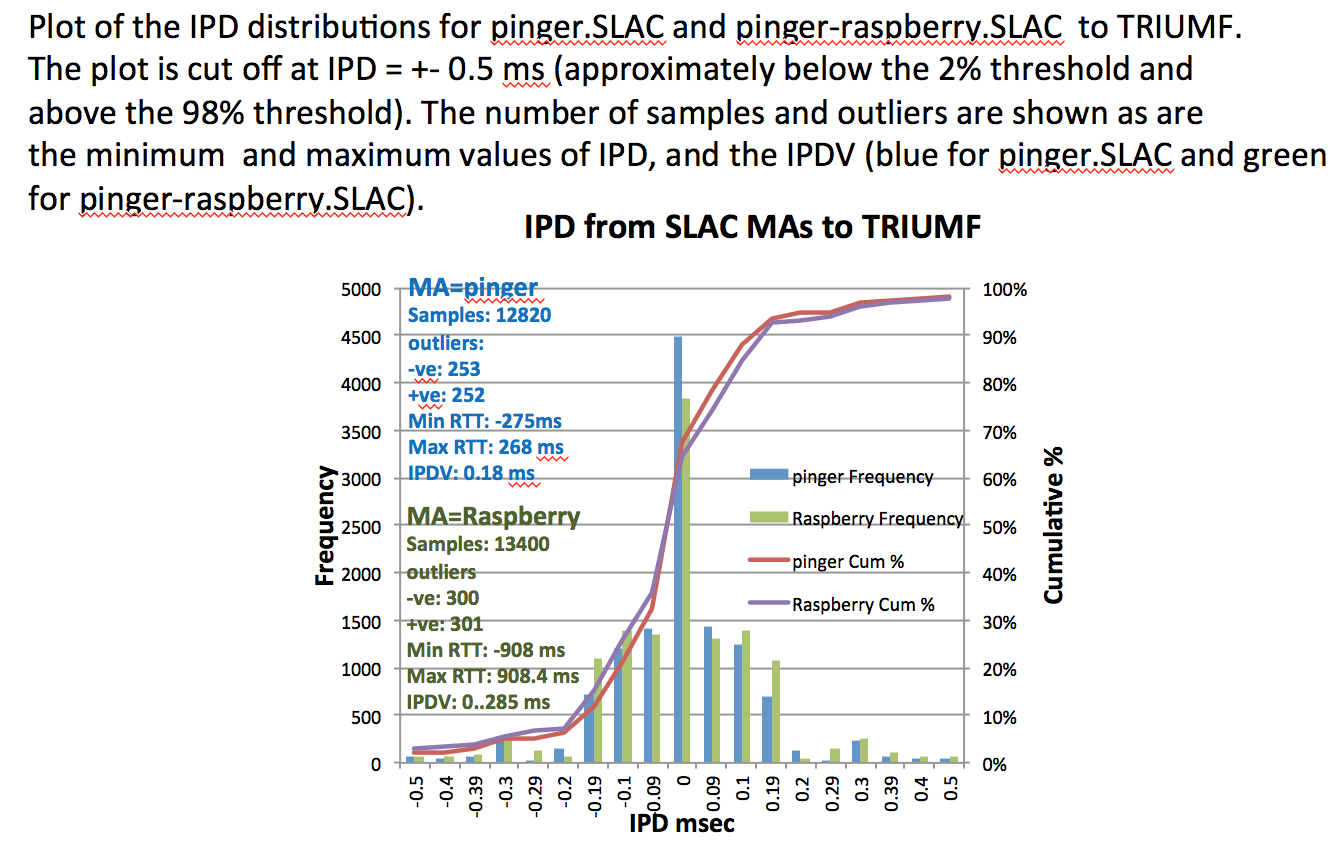
IPD distributions are centered on 0ms and have very wide tails. The one in the figure is cut off below the 2 percentile and above the 98% percentile. The number of outliers not shown is given in the figure, as are the maximum and minimum values of IPD. The distribution is thus seen to have very positive and negative tails. Also as illustrated in the figure a typical IPD distribution has a very sharp peak. To derive the IPDV we take the IQR of the IPD dsitribution. The values for the IPDV for the various measurements are shown in the followjng table; The errors(S) in the IPD are taken from the IQR for the hourly PingER IPDVs observed for the same period. It is seen that the Z-Test in this indicates a value of < 2.0. Assuming the Z-Test is relevant for the non-normal IPD distributions if one uses the IQRs instead of the standard deviation, a value of < 2 for the Z-test statistics indicates the two samples are the same (see http://homework.uoregon.edu/pub/class/es202/ztest.html.
Localhost comparisons
To try and determine more closely the impact of the host on the measuremensts we measured to the localhost NIC port from August 9th to August 19th. Looking at the time series it is apparent that:
- the pinger hosts has considerably shorter RTTs
- the pinger host has fewer large RTT outliers
Looking at the RTT frequency distributions it is apparent that:
- the pinger host's Median RTT is 7 times smaller (0.03ms vs 0.2 ms) than that of the raspberry-pi
- the pinger host's maximum outlier (0.174ms) his ~ factor 60 smaller.
- the pinger host exhibits a pronounced bimodaility not seen for the raspberry-pi.
- The IQRs are very similar (0.025 vs 0.020ms)
| pinger.slac.stanford.edu | pinger-raspberry.slac.stanford.edu | |
|---|---|---|
| Time series | 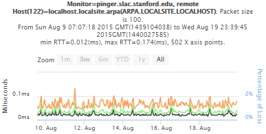 | 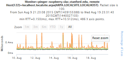 |
| RTT frequency | 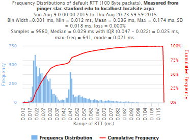 | 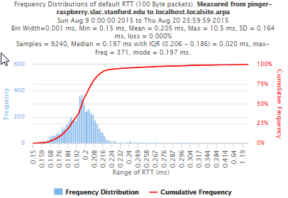 |
| IPD frequency | 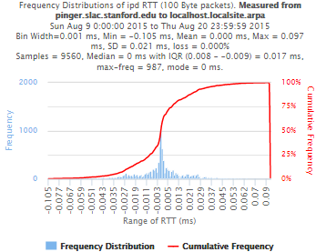 | 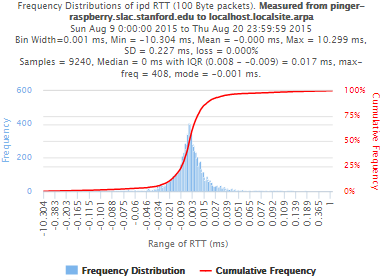 |
Kolmogorov-Smirnov Test
The Kolmogorov-Smirnov test (KS-test) tries to determine if two datasets differ significantly. The KS-test has the advantage of making no assumption about the distribution of data. In other words it is non-parametric and distribution free. The method is explained here and makes use of an Excel tool called "Real Statiscs". The tests were made using the raw data and distributions, both methods had similar results except for the 100Bytes Packet that had a great difference in the results. The results using raw data says both samples does not come from the same distribution with a significant difference, however if we use distributions the result says that only the 1000Bytes packet does not come from the same distribution. Below you will find the graphs for the distributions that were created and the cumulative frequency in both cases plotted one above other (in order to see the difference between the distributions).
| Raw data - 100 Packets | Distribution - 100 Packets | Raw data - 1000 Packets | Distribution - 1000 Packets | |
|---|---|---|---|---|
| D-stat | 0.194674 | 0.039323 | 0.205525 | 0.194379 |
| P-value | 4.57E-14 | 0.551089 | 2.07E-14 | 7.32E-14 |
| D-crit | 0.0667 | 0.067051 | 0.0667 | 0.067051 |
| Size of Raspberry | 816 | 816 | 816 | 816 |
| Size of Pinger | 822 | 822 | 822 | 822 |
| Alpha | 0.05i | |||
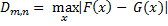
If D-stat is greater than D-crit the samples are not considerated from the same distribution with a (1-Alpha) of accuracy. Remember that D-stat is the maximum difference between the two cumulative frequency curves.
Source: http://www.real-statistics.com/non-parametric-tests/two-sample-kolmogorov-smirnov-test/
In these links you can find the files containing the graphs, histograms and the complete analysis for Kolmogorov-Smirnov between Pinger and Pinger-Raspberry and for SITKA.
Futures
Extension to Android systems
...