...
This document is the basis of a paper comparing (SLAC-PUB-16343) comparing PingER performance on a 1 U bare metal host to that on a Raspberry Pi. It has been running successfuly since July 2015.
This is a project suggested by Bebo White to build and validate a PingER Measurement Agent (MA) based on an inexpensive piece of hardware called a Raspberry Pi (see more about Raspberry Pi) using a linux distribution as the Operating System (see more about Raspbian). If successful one could consider using these in production: reducing the costs, power drain (they draw about 2W of 5V DC power compared to typically over 100W for a deskside computer or 20W for a laptop) and space (credit card size). This is the same type of power required for a smartphone so appropriate off the shelf products including a battery and solar cells are becoming readily available. Thus the Raspberry could be very valuable for sites in developing countries where cost, power utilization and to a lesser extent space may be crucial.
...
- The Raspberry Pi PingER MA must be robust and reliable. It needs to run for months to years with no need for intervention . This still needs to be verified, so far the Raspberry Pi has successfully run without intervention for over a month. This has included and needs automatic recovery after two test power outages.
- The important metrics derived from the measurements made by the Raspberry Pi should not be significantly different from those made by a bare metal PingER MA, or if they are then this needs to be understood.
- The For applications where there is no reliable power siource, the Raspberry Pi needs to be able to run 24 hours a day with only solar derived power. Let's say the power required is 3W at 5V or (3/5)A=0.6A. If we have a 10,000 mAh battery, then at 0.6A it should have power for 10Ah/0.6A ~ 16.6 hours. Then we need a solar cell to be able to refill the battery in a few hours of sunlight. Let's take a 20W 5 V solar panel (see http://www.amazon.com/SUNKINGDOM-trade-Foldable-Charger-Compatible/dp/B00MTEDTWG) = 20/5= 4 A solar panel. So initial guess is 10A-h/4A = 2.5hours. But inefficiences (see http://www.voltaicsystems.com/blog/estimating-battery-charge-time-from-solar/) of say 2.5 extends this to 6.25 hours.
...
PingER measurements are made by ~60 MAs in 23 countries. They make measurements to over 700 targets in ~ 160 countries containing more than 99% of the world's connected population. The measurement cycle is scheduled at roughly 30 minute intervals. The actual scheduled timing of a measurement is deliberately randomized so measurements from one MA are not synchronized with another MA. Typical absolute separation of the timestamp of a measurement from say pinger.slac.stanford.edu to sitka.triumf.ca versus pinger-raspberry.slac.stanford.edu to sitka.triumf.ca is several minutes (e.g. ~ 8 mins for measurements during the time frame June 17 to July 14, 2015), see spreadsheet. At each measurement cycle, each MA issues a set of 100 Byte pings and a set of 1000 Byte ping requests to each target in the MA’s list of targets, stopping when the MA receives 10 ping responses or it has issued 30 ping requests. The number of ping responses is referred to as N and is in the range 0 - 10. The data recorded for each set of pings consists of: the MA and target names and IP addresses; a time-stamp; the number of bytes in the ping request; the number of ping requests and responses (N); the minimum Round Trip Time (RTT) (Min_RTT), the average RTT (Avg_RTT) and maximum RTT (Max_RTT) of the N ping responses; followed by the N ping sequence numbers, followed by the N RTTs. From the N RTTs we derive various metrics including: the minimum ping RTT; average RTT; maximum RTT; standard deviation (stdev) of RTTs, 25% probability (first quartile) of RTT; 75% probability (third quartile) of RTT; Inter Quartile Range (IQR); loss; and reachability (host is unreachable if it gets 100 % loss). We also derive the Inter Packet delay (IPD) and the Inter Packet Delay Variability (IPDV) as the IQR of the IPDs.
...
- The Min RTT error is the IQR of the minimum RTTs from each set of pings for the time period.
- The Avg RTT error is the standard deviation of all the average RTTs from each set of pings for the time period
- The Median RTT error is the IQR of all the individual RTTs from all sets of measurements for the time period
- The IQR IPD IPDV error is the IQR of the hourly IQRs for the time period (see Spreadsheet)
| Metric \ Monitor Target | pinger to pinger-raspberry | pinger-raspberry to pinger | pinger to sitka | pinger-raspberry to sitka | sitka to pinger | sitka to pinger-raspberry | pinger to CERN | pinger-raspberry to CERN |
|---|---|---|---|---|---|---|---|---|
| Time period | June 17 - July 13, 2015 | June 17 - July 13, 2015 | June 17 - July 14, 2015 | June 17 - July 14 | July 15 - July 16 2015 | July 15 - July 16 2015 | June 17 - July 12, 2015 | June 17 - July 12, 2015 |
| Samples | 10890 | 10850 | 10900 | 10850 | 820 | 820 | 10900 | 10900 |
Min RTT | 0.43 ms | 0.41 ms | 22 +- 1 ms | 22.3 +- 1 ms | 22 ms | 22.4 ms | 150 +- 1 ms | 151 ms |
| Avg RTT | 0.542 +- 0.06 ms | 0.529 +- 0.5ms | 23.9 +- 1ms | 23.827 +- 1 ms | 22.30 ms | 22.709 ms | 150.307 +- 2.4 ms | 151.024 +- 1.3 ms |
Max RTT | 1.15 ms | 20.8 ms | 761 ms | 334 ms | 26.3 ms | 25.9 ms | 288 ms | 183 ms |
| Stdev | 0.055 ms | 0.540 ms | 9.58 ms | 9.60 ms | 0.219 ms | 0.222 ms | 2.37 ms | 1.3 ms |
| Median RTT | 0.542 +- 0.05 ms | 0.51 ms +- 0.052 ms | 22.3 +- 0.2 ms | 22.7 +- 0.11 ms | 22.3 +- 0.11 ms | 22.7 +- 0.21 ms | 150 +- 1 ms | 151 +- 0.01 ms |
| 25% | 0.514 ms | 0.48 ms | 22.2 ms | 22.69 ms | 22.3 ms | 22.8 ms | 149.99 ms | 150.99 ms |
| 75% | 0.564 ms | 0.532 ms | 22.4 ms | 22.8 ms | 22.19 ms | 22.59 ms | 151 ms | 151 ms |
| IQR | 0.05 ms | 0.052 ms | 0.2 ms | 0.11 ms | 0.113 ms | 0.210 ms | 1.01 ms | 0.01 ms |
| Min IPD | -0.59 ms | -20.29 ms | -244 ms | -235.1 ms | -0.4 ms | -0.39 ms | -137 ms | -32 ms |
| Avg IPD | 0 ms | 0 ms | 0 ms | 0 ms | 0 ms | 0 ms | 0 ms | 0 |
| Max IPD | 0.62 ms | 20.26 ms | 268 ms | 146 ms | 3.6 ms | 3.29 ms | 138 ms | 32 ms |
| Median IPD | 0 +- 0.07 ms | 0 +- 0.05 ms | 0 +- 0.2 ms | 0 +- 0.2ms | 0 ms +- 0.2 ms | 0 +- 0.2 ms | 0 +- 0.01 ms | 0 +- 0.01 ms |
| Stdev | 0.248 ms | 0.296 ms | ||||||
| 25% IPD | -0.04 ms | -0.03 ms | -0.1 ms | -0.11 ms | -0.1 ms | -0.1 ms | -0.01 ms | -0.01 ms |
| 75% IPD | 0.03 ms | 0.02 ms | 0.09 ms | 0.1 ms | 0.01 ms | 0.09 ms | 0 ms | 0 ms |
| IQR IPD | 0.07 ms | 0.05 ms | 0.190 +- 0.5 ms | 0.210 +- 0.4 ms | 0.2 ms | 0.190ms | 0.01 ms | 0.01 ms |
| Min(abs(IPD)) | 0 ms | 0 ms | 0 ms | 0 ms | 0 ms | 0 ms | 0 ms | 0 ms |
| Avg(abs(IPD)) | 0.041 ms | 0.066 ms | 0.424 ms | 0.406 ms | 0.120 ms | 0.139 ms | 0.386 ms | 0.046 ms |
| Max(abs(IPD)) | 0.0628ms | 20.294 ms | 268 ms | 235.1 ms | 4 ms | 3.29 ms | 138 ms | 32 ms |
| Stdev | 0.248 ms | 0.262 ms | ||||||
| Median(abs(IPD)) | 0.03ms | 0.024 ms | 0.09 ms | 0.1 ms | 0.1 ms | 0.09 ms | 0 ms | 0 ms |
| 25%(abs(IPD)) | 0.01ms | 0.008 ms | 0.01 ms | 0.01 ms | -0.01 ms | -0.01 ms | 0.01 ms | 0.01 ms |
| 75%(abs(IPD)) | 0.058 ms | 0.05 ms | 0.1 ms | 0.19 ms | 0.1 ms | 0.19 ms | 1 ms | 0 ms |
| IQR(abs(IPD) | 0.048 ms | 0.042 ms | 0.09 ms | 0.11 ms | 0.11 ms | 0.2 ms | 0.009 ms | 0.01 ms |
| Loss | 0% | 0% | 0% | 0.008% | 0% | 0% | 0% | 0% |
Since the timestamps of measurements for one MA to a target are not synchronized with another MA to the same target, they are sampling the network at different times. Thus we decided not to use the residuals in the RTTs between on one pair and another. To find the probability of the distributions overlapping use a nomogram of Typically the difference in the time of a measurement from say pinger.slac.stanford.edu to sitka.triumf.ca versus pinger-raspberry.slac.stanford.edu to sitka.triumf.ca averages at 8 mins (see spreadsheet mtr-localhost tab diff mtr).
To find the probability of the distributions overlapping we can use a nomogram of mean differences versus error ratios given in Overlapping Normal Distributions. John M. Linacre for normal distributions. However this does not cover the range we are interested in.
We also use used the Z Tests
Kolmogorov-Smirnov Test
to compare two samples, see for example “Comparing distributions: Z test” available at http://homework.uoregon.edu/pub/class/es202/ztest.html
Spreadsheet (ipdv-errors) has min/avg/max, % and loss between and from pinger & pi to & from sitka, and to cern, plus histograms probabilities, IPDV errors.
Spreadsheet (prob) (Probability table as submitted, IPDV from SLAC to TRIUMF. Also images of IPD graphs from frequency.pl. The IPD distribution from pinger to SLAC has the figure below.
However the ping distributions are decidedly non-normal (see for example the figure below) have wide outliers, and are heavy tailed on the upper side (see https://www.slac.stanford.edu/comp/net/wan-mon/ping-hi-stat.html). This leads to large standard deviations (one to two order of magnitude greater than the IQR) in the RTT values. As can be seen from the table this results in low values of the Z-test and a false probability of no significant statistical difference. Using the IQRs of the frequency distributions instead generally leads to much higher values of the Z-test and hence a higher probability that the distributions of RTTs between two pairs of hosts are significantly different. Comparing the frequency distributions it is seen that there is indeed a marked offset in the RTT values of the peak frequencies and a resultant difference in the cumulative RTT distributions, Using the non-parametric Kolomogorov Smirnoff test (KS test) also indicated significant differences in the distributions.
Average RTTs from pinger.SLAC and pinger-raspberry.slac to TRIUMF (Figure can be found in https://confluence.slac.stanford.edu/download/attachments/192190786/ipdv-errors.xls) The plot cuts off at about the cumulative 98%. The number of overflows not plotted are indicated. |
|---|
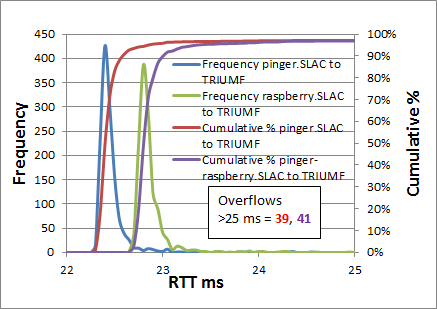 |
The RTT measurements made from pinger.SLAC and pinger-raspberry.SLAC to TRIUMF and CERN average around 23ms and 151ms respectively. Despite this large difference in average RTTs', comparing the average RTTs from pinger.SLAC with those from pinger-raspberry.SLAC yields a difference of only ~0.35ms for both TRIUMF and CERN.
Looking at the traceroutes, using Matt's traceroute to measure the RTT to each hop, indicates that this difference starts at the first hop and persists for later hops. See spreadsheet (MTR tab). We therefore made ping measurements from each SLAC MA to its loopback network interface. The measurements were made at the same times to facilitate comparisons. They indicate that the pinger-raspberry.SLAC is ~0.13ms lslower in responding than the pinger.SLAC MA. Thus approximately 1/3rd of the difference in average RTS tro TRIUMF measured by the two SLAC MAs is due to the MA platform itself.
IPDV
PingER's main metric for measuring jitter is the IPDV. A typical IPD distribution from which the IPD is derived is shown below.
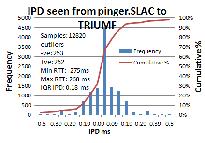
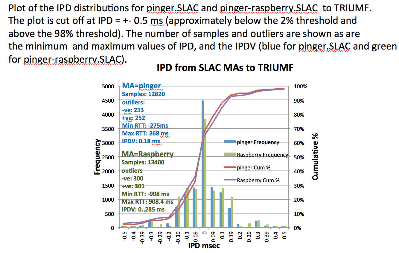
IPD distributions are centered on 0ms and have very wide tails. The one in the figure is cut off below the 2 percentile and above the 98% percentile. The number of outliers not shown is given in the figure, as are the maximum and minimum values of IPD. The distribution is thus seen to have very positive and negative tails. Also as illustrated in the figure a typical IPD distribution has a very sharp peak. To derive the IPDV we take the IQR of the IPD dsitribution. The values for the IPDV for the various measurements are shown in the followjng table; The errors(S) in the IPD are taken from the IQR for the hourly PingER IPDVs observed for the same period. It is seen that the Z-Test in this indicates a value of < 2.0. Assuming the Z-Test is relevant for the non-normal IPD distributions if one uses the IQRs instead of the standard deviation, a value of < 2 for the Z-test statistics indicates the two samples are the same (see http://homework.uoregon.edu/pub/class/es202/ztest.html.
Localhost comparisons
To try and determine more closely the impact of the host on the measurements, we eliminated the effect of the network by making measurements to the host's localhost NIC port. Looking at the analyzed data it is apparent that:
- the pinger hosts has considerably shorter RTTs
- the pinger host has fewer large RTT outliers
Looking at the RTT frequency distributions it is apparent that:
- the pinger and raspberry host RTT frequency distributions hardly overlap at all (one sample (0.04%) of the raspberry pi distribution overlaps ~ 7% of the pinger distribution).
- the pinger host's Median RTT is 7 times smaller (0.03ms vs 0.2 ms) than that of the raspberry-pi
- the pinger host's maximum outlier (0.174ms) is ~ factor 60 smaller than the raspberry-pi.
- the pinger host exhibits a pronounced bimodaility not seen for the raspberry-pi.
- the IQRs are very similar (0.025 vs 0.020ms)
Looking at the IPD distributions it is apparent that:
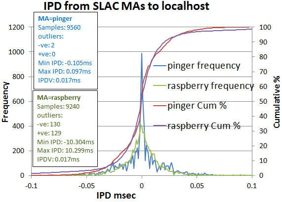
- the pinger distribution is much sharper (max frequency 987 vs 408 for raspberry-pi)
- there is a slight hint of multi-modaility in the pinger distribution less visible in the raspberry-pi distribution
- the minimum and maximum outliers are about a factor 100 lower for pinger than the raspberry-pi (~ +-0.1 vs ~10ms)
- the IPDV's are similar (0.017ms), whereas the standard deviations differ by almost a factor of 10 (0.021ms vs. 0.227ms. This further illustrates the impact of smaller outliers seen by pinger.
Comparing the IPD frequency distributions for the pinger.SLAC and pinger-raspberry MAs to their localhosts with those to TRIUMF it is seen that the differences are washed out as one goes to the longer RTTs.
Though there are large relative differences in the distributions, the absolute differences of the aggregated statistics (medians, IQRs) are sub millisecond and so should not noticeably affect PingER wide area network results.
Though we have not analyzed the exact reason for the relative differences, we make the following observations:
- The factor of 7 difference in the median RTTs is probably at least partially related to the factor ten in the NICs (1Gbps vs 100Mbps) and the factor of 5 difference in the clock speeds (3Ghz vs 600MHz).
- Looking at the minimum RTTs for each set of pings it is seen that pinger has a larger ratio of median RTT / IQR compared to the raspberry-pi (0.33 vs 0.096).
- This may be related to the fact that the pinger host is less dedicated to acting as a PingER MA since in addition it runs lots of cronjobs to gather, archive and analyze the data. This may also account for some of the more pronounced multi-modality of the pinger host's RTT distributions.
- Currently we do not have a rationale for the reduced outliers on pinger vs the raspberry-pi.
| pinger.slac.stanford.edu | pinger-raspberry.slac.stanford.edu | |
|---|---|---|
| Time series | 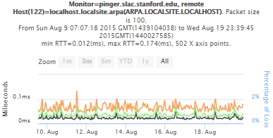 | 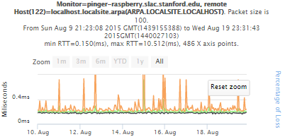 |
| RTT frequency | 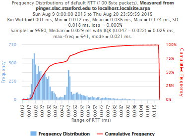 | 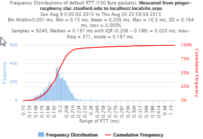 |
| Minimum RTTs for each set of 10 pings | 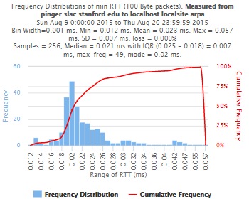 | 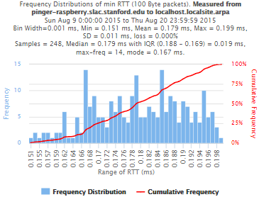 |
| IPD frequency | 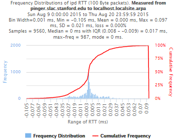 | 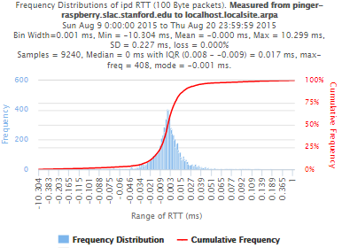 |
Kolmogorov-Smirnov Test
The Kolmogorov-Smirnov test (KS-test) tries to determine if two datasets differ significantly. The KS-test has the advantage of making no assumption about the distribution of data. In other words it is non-parametric and The Kolmogorov-Smirnov test (KS-test) tries to determine if two datasets differ significantly. The KS-test has the advantage of making no assumption about the distribution of data. In other words it is non-parametric and distribution free. The method is explained here and makes use of an Excel tool called "Real Statiscs". The tests were made using the raw data and distributions, both methods had similar results except for the 100Bytes Packet that had a great difference in the results. The results using raw data says both samples does not come from the same distribution with a significant difference, however if we use distributions the result says that only the 1000Bytes packet does not come from the same distribution. Bellow Below you will find the graphs for the distributions that were created and the cumulative frequency in both cases plotted one above other (in order to see the difference between the distributions).
| Raw data - 100 Packets | Distribution - 100 Packets | Raw data - 1000 Packets | Distribution - 1000 Packets | |
|---|---|---|---|---|
| D-stat | 0.194674 | 0.039323 | 0.205525 | 0.194379 |
| P-value | 4.57E-14 | 0.551089 | 2.07E-14 | 7.32E-14 |
| D-crit | 0.0667 | 0.067051 | 0.0667 | 0.067051 |
| Size of Raspberry | 816 | 816 | 816 | 816 |
| Size of Pinger | 822 | 822 | 822 | 822 |
| Alpha | 0.05 | |||
If D-stat is greater than D-crit the samples are not considerated from the same distribution with a (1-Alpha) of accuracy. Remember that D-stat is the maximum difference between the two cumulative frequency curves.
Source: http://www.real-statistics.com/non-parametric-tests/two-sample-kolmogorov-smirnov-test/
Futures
Extension to Android systems
Topher: Here is where we would like you to say something about the potential Android opportunity.
Installation process
The installation procedures for a PingER MA are relatively simple, but do require a Unix knowledgeable person to do the install and it typically takes a couple hours and may require a few corrections pointed out by the central PingER admin. It is possible to pre-configure the Raspberry Pi at the central site and ship it pre-configured to the MA site. However that requires funding the central site Raspberry Pi acquisitions, may raise issues of on-going commitment, and may not be acceptable for the Cyber security folks at the MA site. We are looking at simplifying the install process, possibly by creating an ISO Image
Robustness and Reliability
| 0.039323 | 0.205525 | 0.194379 | ||
| P-value | 4.57E-14 | 0.551089 | 2.07E-14 | 7.32E-14 |
| D-crit | 0.0667 | 0.067051 | 0.0667 | 0.067051 |
| Size of Raspberry | 816 | 816 | 816 | 816 |
| Size of Pinger | 822 | 822 | 822 | 822 |
| Alpha | 0.05i | |||
If D-stat is greater than D-crit the samples are not considered from the same distribution with a (1-Alpha) of accuracy. Remember that D-stat is the maximum difference between the two cumulative frequency curves.
Source: http://www.real-statistics.com/non-parametric-tests/two-sample-kolmogorov-smirnov-test/
In these links you can find the files containing the graphs, histograms and the complete analysis for Kolmogorov-Smirnov between Pinger and Pinger-Raspberry and for SITKAThis still needs to be demonstrated in the field. We also need to more fully understand the solar power requirements.