| Table of Contents | ||||||
|---|---|---|---|---|---|---|
|
Introduction
Omega3P is a parallel finite-element electrogmagnetic code for high-fidelity modeling of cavities. It calculates the resonant frequencies and other rf parameters of a cavity, as well as damping effects due to external couplings. It uses Nedelec-type hierarchical vector basis up to 6th order with quadratic (10-points) tetrahedral elements for improved solution accuracy.
Mathematical Modeling
Lossless cavities
Maxwell's equations in the frequency domain for a perfectly conducting cavity can be written as the following PDE,
| Wiki Markup |
|---|
| Wiki Markup |
{toc:outline=true|indent=0px|minLevel=2} h2. Introduction Omega3P is a parallel finite-element electrogmagnetic code for high-fidelity modeling of cavities. It calculates the resonant frequencies and other rf parameters of a cavity, as well as damping effects due to external couplings. It uses Nedelec-type hierarchical vector basis up to 6th order with quadratic (10-points) tetrahedral elements for improved solution accuracy. h2. Mathematical Modeling h3. Lossless cavities Maxwell's equations in the frequency domain for a perfectly conducting cavity can be written as the following PDE, {center:class=myclass} {latex} \begin{eqnarray*} \nabla \times \left(\frac{1}{\mu} \nabla \times \vec{\mathbf E}\right) - k^2 \epsilon \vec{\mathbf E} & = 0 & on \quad \Omega \\ \vec{\mathbf n} \times \vec{\mathbf E} & = 0 & on \quad \Gamma_{E} \\ \vec{\mathbf n} \times \left( \frac{1}{\mu} \nabla \times \vec{\mathbf E} \right) & = 0 & on \quad \Gamma_{M} \\ \end{eqnarray*} {latex} {center} |
We
...
use
...
Neelec-type
...
vector
...
basis
...
functions
...
to
...
discretize
...
the
...
electric
...
field:
| Wiki Markup |
|---|
{center:class=myclass} {latex}\[\vec{\mathbf E}=\sum_i x_i \vec{\mathbf N}_i\]{latex} {center} |
We
...
obtain
...
the
...
following
...
generalized
...
eigenvalue problem:
| Wiki Markup |
|---|
{center:class=myclass} problem: {latex} \begin{eqnarray*} {\mathbf Kx} = k^2 {\mathbf Mx} \quad where & \\ {\mathbf K}_{ij} = \int_{\Omega} \left( \nabla \times \vec{\mathbf N}_i \right) \cdot \frac{1}{\mu} \left( \nabla \times \vec{\mathbf N}_j \right) d\Omega & \\ {\mathbf M}_{ij} = \int_{\Omega} \vec{\mathbf N}_i \cdot \epsilon \vec{\mathbf N}_j d\Omega & \\ \end{eqnarray*} {latex} {center} |
The
...
matrix
...
K
...
is
...
real
...
symmetric
...
while
...
M
...
is
...
real
...
symmetric
...
positive
...
definite.
...
If
...
there
...
are
...
lossy
...
materials
...
in
...
the
...
cavity,
...
the
...
matrix
...
M
...
and/or
...
K
...
will
...
be
...
complex.
...
Waveguide
...
loaded
...
cavities
...
For
...
modeling
...
waveguide-loaded
...
cavities,
...
we
...
use
...
either
...
the
...
absorbing
...
boundary
...
condition
...
(ABC)
...
or
...
the
...
waveguide
...
boundary
...
condition
...
(WBC).
...
The
...
following
...
picture
...
illustrates
...
a
...
cavity
...
with
...
3
...
waveguides,
...
and
...
each
...
of
...
them
...
is
...
modeled
...
with
...
ABC.
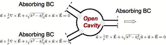
The discretized system is a complex nonlinear eigenvalue problem,
| Wiki Markup |
|---|
{center:class=myclass} !Absorbing.png|width=500,align=center! The discretized system is a complex nonlinear eigenvalue problem, {latex} \[ {\mathbf Kx} + i \sum_j \sqrt{k^2-k^2_{cj}} {\mathbf W}_j {\mathbf x} = k^2 {\mathbf Mx} \] {latex} {center} |
where
...
the
...
damping
...
matrix
...
W is
| Wiki Markup |
|---|
{center:class=myclass}* is {latex} \[ ({\mathbf W}_j)_{mn} = \int_{\Gamma} \left( \vec{\mathbf n} \times \vec{\mathbf N}_m \right) \cdot \left( \vec{\mathbf n} \times \vec{\mathbf N}_n \right) d\Gamma \] {latex}{center} |
The
...
following
...
picture
...
illustrates
...
a
...
cavity
...
with
...
waveguides,
...
which
...
are
...
modeled
...
with
...
WBC.
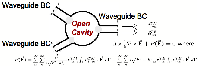
The corresponding discretized system becomes a complex nonlienar eigenvalue problem,
| Wiki Markup |
|---|
{center:class=myclass} !Waveguide.png|align=center,width=500! The corresponding discretized system becomes a complex nonlienar eigenvalue problem, {latex} \[ {\mathbf Kx} + i \sum_{m,n} \sqrt{k^2-(k^{TE}_{mn})^2} {\mathbf W}^{TE}_{mn} {\mathbf x} + i \sum_{m,n} \frac{k^2}{\sqrt{k^2-(k^{TM}_{mn})^2}} {\mathbf W}^{TM}_{mn} {\mathbf x} = k^2 {\mathbf Mx} \] {latex}{center} |
where
...
the
...
waveguide
...
matrices are
| Wiki Markup |
|---|
{center:class=myclass} are {latex} \[ ({\mathbf W}^{TE}_{mn})_{ij} = \int_{\Gamma} \vec{\mathbf e}^{TE}_{mn} \cdot \vec{\mathbf N}_i d\Gamma \int_{\Gamma} \vec{\mathbf e}^{TE}_{mn} \cdot \vec{\mathbf N}_j d\Gamma \] \\ \[ ({\mathbf W}^{TM}_{mn})_{ij} = \int_{\Gamma} \vec{\mathbf e}^{TM}_{tmn} \cdot \vec{\mathbf N}_i d\Gamma \int_{\Gamma} \vec{\mathbf e}^{TM}_{tmn} \cdot \vec{\mathbf N}_j d\Gamma \] {latex} h2. Numerical Methods The following is a graphical description of the four different types of physics problems that Omega3P can solve and the solver options that can be used.{center} |
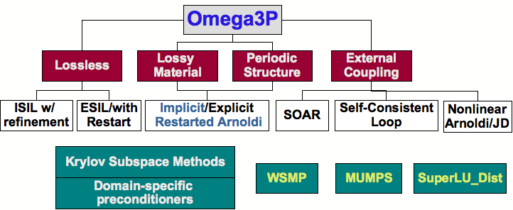
Numerical Methods
The following is a graphical description of the four different types of physics problems that Omega3P can solve and the solver options that can be used.
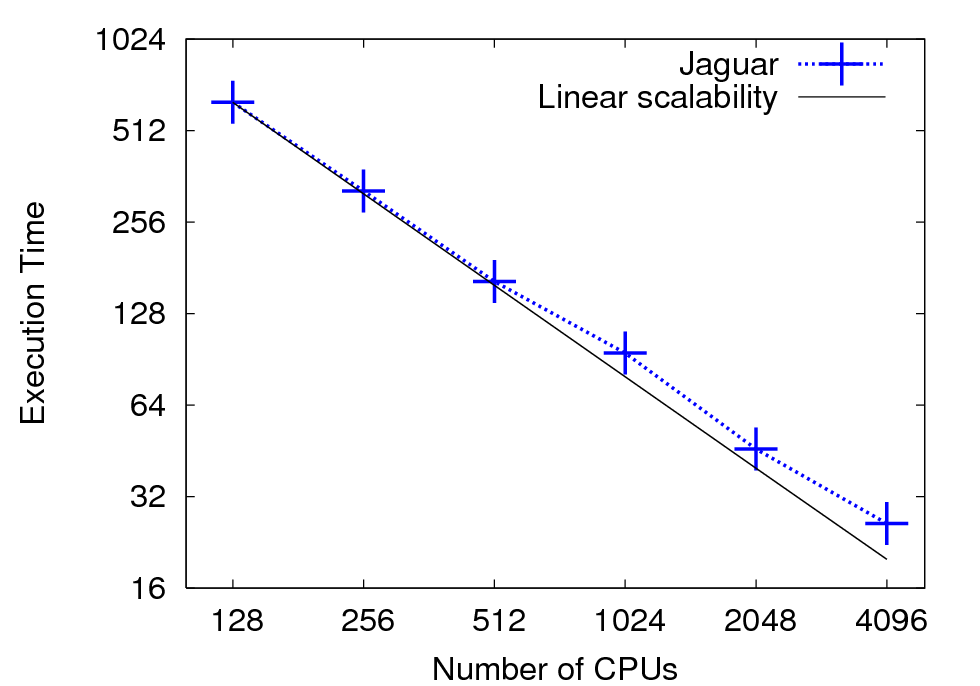
Parallel Performance
Omega3P parallel performance is heavily dependent on the solver used. In general, using sparse direct solvers for shifted linear systems often yields higher FLOPS than using Krylov subspace iterative methods. On the other hand, the latter has much better scalability.
The following is a strong scalability plot for Omega3P running on ORNL Jaguar (Cray XT). It used 1.5 million higher-order tetrahedral elements for the RF gun of the LCLS. . The number of the degrees of freedom is about 9.6 millions, and the number of nonzeros in the resulting matrix about 506 millions. It is shown that Omega3P scales to 4096 number of CPUs with more than 95% of parallel efficiency.