Page History
Contents
| Table of Contents |
|---|
Online Analysis Design
Online Analysis Design - Presentation by Matt for January 2012 DAQ Meeting
...
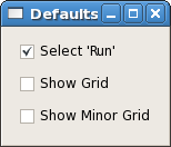
"Defaults" control provides users a feature to set specific settings (show grid/minor grid etc.) of online monitoring plots as default.
Data: This section provides various features for data in various plots. "Reset Plots" control will reset the all displayed plots by clearing their content and restart ploting with new set of data. Users can save plots using "Save Plots" control available in this section. Plot data will be saved as ".dat" file in terms of values associated with its axis.
...
For X-Y plot (Acqiris Digitizer Waveform), contents of saved plot will be saved as value vectors of X and Y axis in a ".dat" file as shown below:
| No Format |
|---|
1.5e-09  0.000561523
2.5e-09  0.000170898
3.5e-09  0.000170898
4.5e-09  0.000366211
5.5e-09  -0.000195313
6.5e-09  0.000268555
7.5e-09  7.32422e-05
8.5e-09  0.000366211
9.5e-09  7.32422e-05
1.05e-08 7.32422e-05
:
:
|
...
The steps to creating a user module are:
Copy /reg/g/pcds/package/amiuser to your area
Code Block cp -rf /reg/g/pcds/package/amiuser ~/.Edit the ExampleAnalysis.{hh,cc} files
Code Block cd ~/amiuser; gedit ExampleAnalysis.ccBuild the libamiuser.so library
Code Block make allCopy the libamiuser.so to your experiment's home area
Code Block cp libamiuser.so ~amoopr/.\\\\
The "~amoopr/libamiuser.so" plug-in module is specified explicitly in the "-L" command-line option for the monitoring executable that appears in /reg/g/pcds/dist/pds/amo/scripts/amo.cnf, for example. It is possible to specify a comma separated list of libraries in the "-L" option to include more than one plug-in module.
The plug-in modules will be picked up the next time the DAQ system is restarted.
The UserModule class contains several member functions that must be implemented:
- clear() - unregister plots and disable analysis
- create() - register plots and enable analysis
- reset(featurecache) - called prior to a new configuration with a reference to the cache of event variables
- clock(timestamp) - called once for each event or configuration
- configure(detectorid, datatype, data*) - called for each detector datum in the configuration
- event(detectorid, datatype, data*) - called for each detector datum in the event
- accept() - called once after all 'event()' callbacks have completed; returns a filter decision
- name() - returns the module name
The 'detectorid' arguments are of the form Pds::Src and may be cast for comparison against detector identities such as Pds::DetInfo or BLD identities such as Pds::BldInfo (Pds:: classes from pdsdata/xtc package). The 'datatype' arguments are of the form Pds::TypeId which is a class denoting the data format (image, waveform, etc., and version, also from pdsdata/xtc package). The 'data*' arguments are pointers to the configuration or event data (from pdsdata/<type> package). For the 'configure' callbacks with relevant data, the data should be copied. For the 'event' callbacks, the pointers may simply be copied and referenced when the 'analyze' function is called.
Six types of plots may be displayed { Strip chart, 1D histogram, 1D profile histogram, waveform, 2D image, 2D scatter plot } by instanciating the ami/data classes { EntryScalar, EntryTH1F, EntryProf, EntryWaveform, EntryImage, EntryScan }, respectively. The interfaces for these classes are found in the corresponding release/ami/data/Entry*.hh files. For example, a 1D histogram is created by generating its description
| Code Block |
|---|
DescTH1F(const char* name, const char* xtitle, const char* ytitle, unsigned nbins, float xlow, float xhigh)
|
as found in release/ami/data/DescTH1F.hh and passing it to the EntryTH1F constructor. For example,
| Code Block |
|---|
DescTH1F desc("My Plot","My X title","My Y title",100, 0., 1.);
EntryTH1F* plot = new EntryTH1F( desc );
|
The plot may be filled by calling its function
| Code Block |
|---|
plot->addcontent(weight, x_value);
|
and validated for display by calling
| Code Block |
|---|
plot->valid();
|
See the examples {ExampleAnalysis.cc, AcqirisAnalysis.cc, CamAnalysis.cc}.
The new plots will appear in a section of the online monitoring with a title matching the 'name()' method of the module. By default a separate page is created for each added plot. Multiple plots may appear in the same tab if their titles end in the same string - '#' followed by a page title; for example, two plots titled 'First energy plot#Energy' and 'Second energy plot#Energy' will appear on a page titled 'Energy' with the individual titles 'First energy plot' and 'Second energy plot'. This should allow users to add a few additional plots using operations not supported by the generic monitoring.
...
To use the example files you will need two shells. The executables are in
release/build/pdsdata/bin/x86_64-linux-dbg. Assuming both shells are in
the executable directory, first start the server with something like:
| Code Block |
|---|
./xtcmonserver -f ../../../../opal1k.xtc -n 4 -s 0x700000 -r 120 -p yourname -c 1 [-l]
|
...
Once the server is started, you can start the client side in the
second shell with:
| Code Block |
|---|
./xtcmonclientexample -p yourname -c clientId
|
...
To write your own monitoring software, all you have to do is subclass the
XtcMonitorClient class and override the XtcMonitorClient::processDgram()
method to supply your own client side processing of the DataGram events
in the XTC stream or file supplied by the file server. Below is the example
implemented by XtcMonClientExample.cc.
| Code Block |
|---|
class MyXtcMonitorClient : public XtcMonitorClient {
  public:
    virtual int processDgram(Dgram* dg) {
      printf("%s transition: time 0x%x/0x%x, payloadSize 0x%x\n",TransitionId::name(dg->seq.service()),
             dg->seq.stamp().fiducials(),dg->seq.stamp().ticks(),dg->xtc.sizeofPayload());
      myLevelIter iter(&(dg->xtc),0);
      iter.iterate();
      return 0;
    };
};
|
...
There is a DAQ Offline Monitoring program that operates just like the Online Monitoring program except that it includes an additional section at the top of the user interface that allows one to select offline runs stored in directories. To use it, log onto a machine that has access to the xtc directories you would like to use as input data. Then, run:
/reg/g/pcds/dist/pds/ami-x.x.x-px.x.x/build/ami/bin/x86_64-linux-opt/offline_ami
where ami-x.x.x-px.x.x should be the most version in the pds directory (3.3.5 ami-8.2.8-p8.2.4 as of this writing).
Click the Select button and the program will bring up a "Select Directory" dialog. Use that to navigate to the directory containing the xtc files you are interested in. For example:
...
Overview
Content Tools