Page History
...
Online Analysis Tutorial - presented at SSRL/LCLS User's conference, 20142014
Online Analysis Design
Online Analysis Design - Presentation by Matt for January 2012 DAQ Meeting
...
| Anchor | ||||
|---|---|---|---|---|
|
Using the Online Monitoring GUI
"Restart DAQ" icon and "Restart Monitoring" icons on operator console brigns bring up multiple GUI panels for DAQ system. Online Monitoring GUI is as shown below:

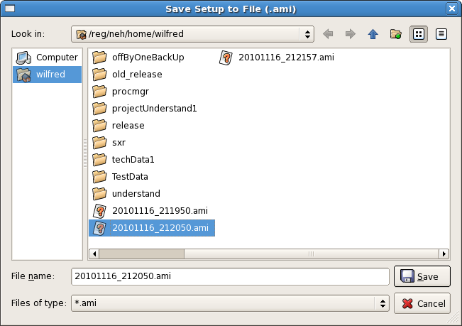
Setup : This section deals with setting up various display windows for online monitoring. "Save" control provides a way to archive configuration of current display windows. (X-Y plots, 2-D frame etc.) Whereas, "Load" control retrives existing display windows configuration. Display configuration is saved in file with extension ".ami" as shown in following figure.
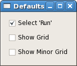
"Defaults" control provides users a feature to set specific settings (show grid/minor grid etc.) of online monitoring plots as default.
Data: This section provides various features for data in various plots. "Reset Plots" control will reset the all displayed plots by clearing their content and restart ploting with new set of data. Users can save plots using "Save Plots" control available in this section. Plot data will be saved as ".dat" file in terms of values associated with its axis.
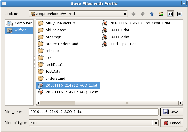
For X-Y plot (Acqiris Digitizer Waveform), contents of saved plot will be saved as value vectors of X and Y axis in a ".dat" file as shown below:
A list of primary event displays is shown in the Data panel of the DAQ Online Monitoring window. This list reflects various detectors involved in the current run of the experiment. A mouse click on specific event display will open up a corresponding data monitoring plot. Each type of data plot has multiple features attched to it which will be covered in following section.The Online Monitoring GUI is shown below:
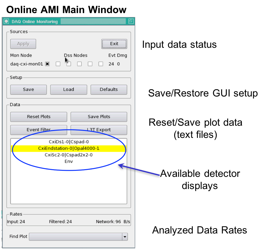
Sources: The Sources panel allows the user to map which monitoring nodes receive events destined for a specific DSS node. In the example above, daq-cxi-mon01 will see the same data that is being recorded by daq-cxi-dss01.
Setup: The Setup panel allows the user to save various display windows and to load a saved setup from a file. "Save" control provides a way to archive configuration of current display windows. (X-Y plots, 2-D frame etc.) Whereas, "Load" control retrives existing display windows configuration. Display configuration is saved in file with extension ".ami" as shown in following figure.
"Defaults" control button provides users a feature to set specific settings (show grid/minor grid etc.) of online monitoring plots as default.
Data: The Data panel shows operations that can be applied to all plots (all data), such as resetting them, applying an event filter, or saving plots. "Reset Plots" control will reset the all displayed plots by clearing their content and restart plotting with a new set of data. Users can save plots using the "Save Plots" button available in this section. Plot data will be saved as a ".dat" file in terms of values associated with its axis.
For X-Y plot (Acqiris Digitizer Waveform), contents of saved plot will be saved as value vectors of X and Y axis in a ".dat" file as shown below:
| No Format |
|---|
1.5e-09  0.000561523
2 |
| No Format |
1.5e-09 0.000561523 2.5e-09 0.000170898 3.5e-09 0.000170898 4.5e-09 0.000366211 5.5e-09 -0.000195313 6.5e-09 0.000268555000170898 73.5e-09 70.32422e-05000170898 84.5e-09 0.000366211 95.5e-09 7.32422e-05 1.05e-08 7.32422e-05 : : |
List of primary event displays is shown at the bottom part of the "Online Monitoring Window". This list reflects various detectors involved in current run of experiment. A mouse click on specic event display will openup corresponding data monitoring plot. Each type of data plots has multiple features attched to it which will be covered in following section.

Details of Scalar variables/data
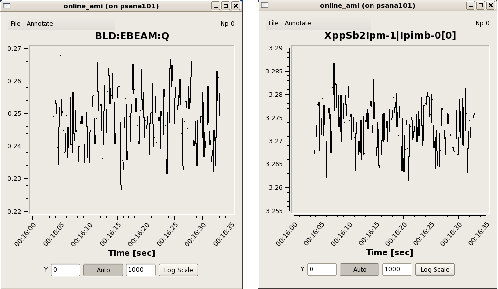
Ebeam and Ipimb data view details
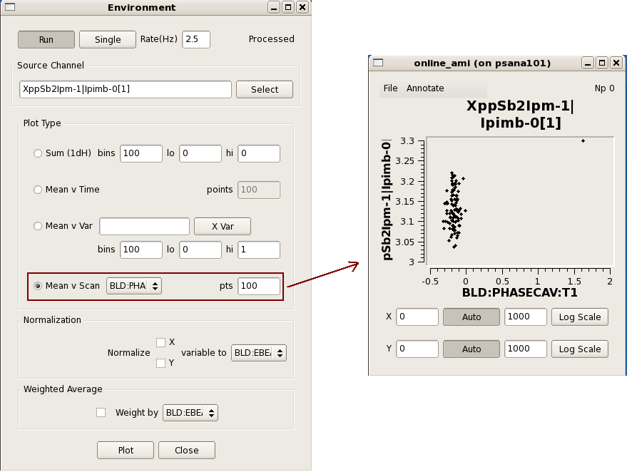
Correlation plots between 2 scalar data object
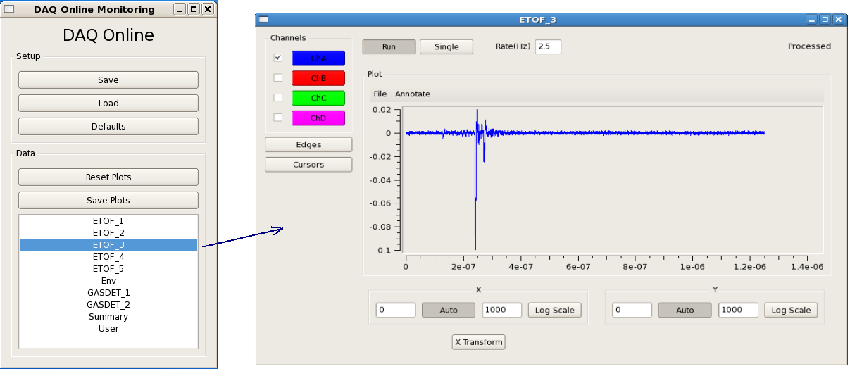
Waveform Display
Acqiris Details
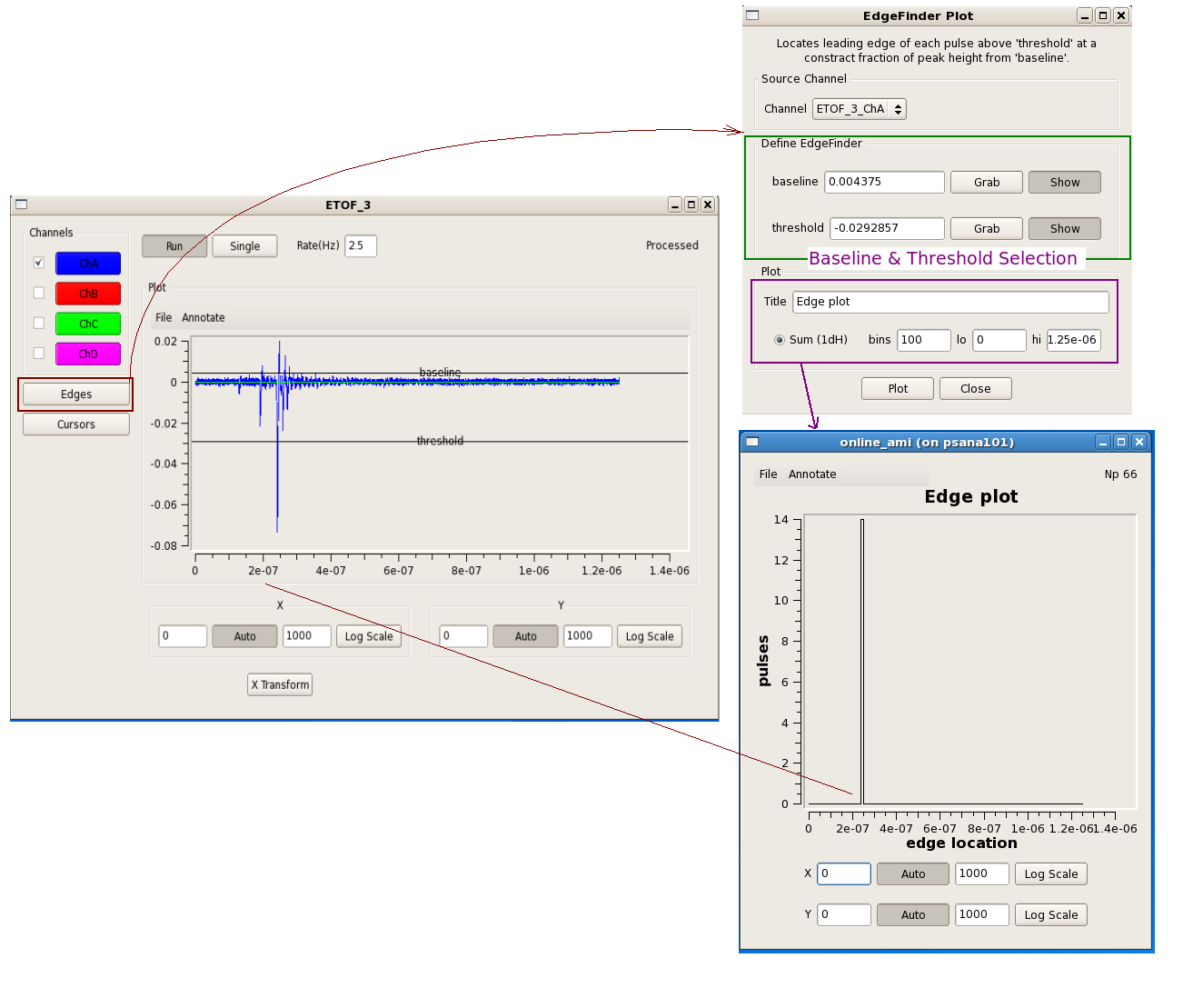
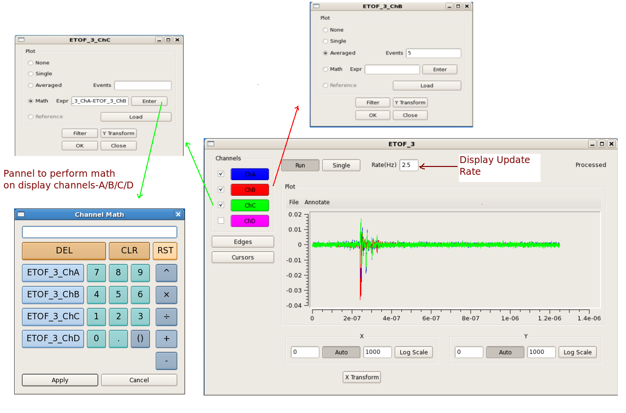
Edge operations
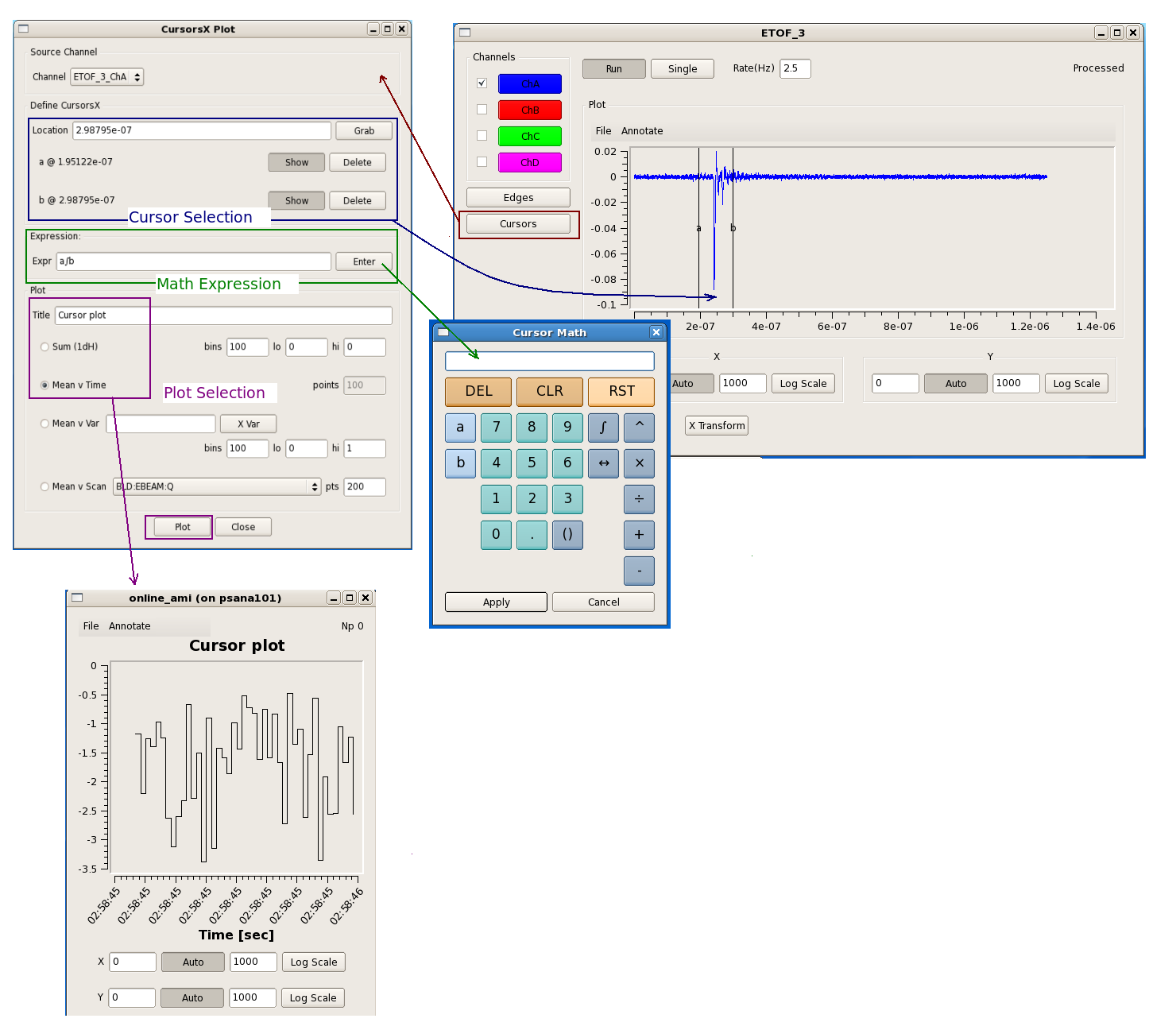
Cursors Operations
Features attched to it which will be covered in following section.
-0.000195313
6.5e-09  0.000268555
7.5e-09  7.32422e-05
8.5e-09  0.000366211
9.5e-09  7.32422e-05
1.05e-08 7.32422e-05
:
:
|
Rates: The Rates panel at the bottom shows the effective input data rate to AMI and the network bandwidth. The Find Plot button helps a user to bring a specific plot to the foreground.
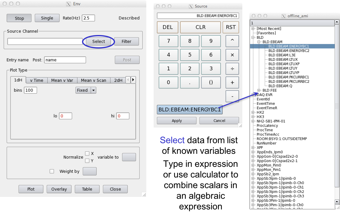
Env Window: Choose Data to Plot
Env or Environment data is all scalar data associated with the event. This includes Event Receiver data, Beamline Data such as the beam energy, phase cavity, and FEE Gas Detector quantities, diode readout values, encoder readout, EPICS variables included in the DAQ data stream, and Posted data, processed detector data for this event (set up elsewhere).
Examples of Scalar variables/data
Ebeam and Ipimb data view details
Correlation plots between 2 scalar data object
Waveform Display
Acqiris Details
Edge operations
Cursors Operations
Features attched to it which will be covered in following section.
Some speciall function buttons on the calculator
Button | Function |
|---|---|
a ∫ b | Integrate from a to b |
a ⨍ b | 1st moment from a to b |
a ⨎ b | 2nd moment from a to b |
a ↔ b | Samples(bins) from a to b |
| Anchor | ||||||
|---|---|---|---|---|---|---|
|
Writing a plug-in to the Online Monitoring GUI
The core online monitoring can be specialized by supplying plug-in modules containing user code. These modules can
(1) compute variables to be used in the monitoring GUI,
(2) generate additional plots to be displayed, and
(3) provide a filtering decision for events to be used in the monitoring.
...
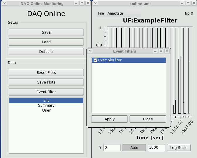
The new plots will appear in a section of the online monitoring with a title matching the 'name()' method of the module. By default a separate page is created for each added plot. Multiple plots may appear in the same tab if their titles end in the same string - '#' followed by a page title; for example, two plots titled 'First energy plot#Energy' and 'Second energy plot#Energy' will appear on a page titled 'Energy' with the individual titles 'First energy plot' and 'Second energy plot'. This should allow users to add a few additional plots using operations not supported by the generic monitoring.
The module names will also appear in the 'Event Filters' section of the online monitoring for selection as global filters, and any added variable names will appear in the 'Env' section of the monitoring for use as inputs to other plots. This should allow users to improve the generic monitoring for infrequent or specially classified events. It is also a testbed for how users may be able to reduce recorded data volumes, if so desired.
...
'Energy' with the individual titles 'First energy plot' and 'Second energy plot'. This should allow users to add a few additional plots using operations not supported by the generic monitoring.
The module names will also appear in the 'Event Filters' section of the online monitoring for selection as global filters, and any added variable names will appear in the 'Env' section of the monitoring for use as inputs to other plots. This should allow users to improve the generic monitoring for infrequent or specially classified events. It is also a testbed for how users may be able to reduce recorded data volumes, if so desired.
| Anchor | ||||
|---|---|---|---|---|
|
Writing a user application that reads from shared memory
If you wish to write a user application that reads from shared memory, it is recommended that you get in touch with the hutch point-of-contact for assistance. AMI and psana can both read from shared memory and most analyses can be accomplished within one of the two frameworks.
The shared memory server can either support 1 or multiple clients, depending on the command line flags passed in when the server is launched. Events can be handed to multiple clients in a round-robin style (useful for parallelism) or every client can see all events. Multiple shared memory servers can run on one monitoring node, but each server must have a unique name for its block of memory (seen in /dev/shm).
| Code Block |
|---|
Usage: monshmserver -p <platform> -P <partition> -i <node mask> -n <numb shm buffers> -s <shm buffer size> [options]
Options: -q <# event queues>  (number of queues to hold for clients)
         -t <tag name>        (name of shared memory)
         -d                   (distribute events)
         -c                   (allow remote control of node mask)
         -g <max groups>      (number of event nodes receiving data)
         -T <drop prob>       (test mode - drop transitions)
-h |
Shared memory server flags:
- -c: indicates a shared memory server whose dss node mapping can be dynamically changed. (The psana monshmservers should not have the "-c" flag.)
- -d: distribute each event to a unique clients (other option is all clients are given the same event). A faster client will receive more events in "-d" mode.
-i: bitmask specifying multicast groups (i.e. which dss node's data we see)
-n: total number of buffers. if there are 8 clients, and 8 buffers, each client gets 1 buffer.
- -q: maximum number of clients ("queues") that this shared memory server will send events to
- -s: the buffer size (in bytes) reserved for each event. the event has to fit in this space. if the product of this number and the argument to "-n" is too large, the software can crash because a system shared memory limit has been exceeded.
- -t: "name" of the shared memory (e.g. the "psana" in DataSource('shmem=psana.0:stop=no')
- -P: the partition name used to construct the name of the shared memory. c
The shared memory server can be restarted with a command similar to this:
/reg/g/pcds/dist/pds/tools/procmgr/procmgr restart /reg/g/pcds/dist/pds/cxi/scripts/cxi.cnf monshmsrvpsana |
The last argument is the name of the process which can be found by reading the .cnf file (the previous argument). This command must be run by the same user/machine that the DAQ used to start all its processes (e.g. for CXI it was user "cxiopr" on machine "cxi-daq"). If a shared-memory server is restarted, it loses its cached "configure/beginrun/begcalib" transitions, so the DAQ must redo those transitions for the server to function correctly.
To find out the name of the shared memory segment on a given monitoring node, do something similar to the following:
[cpo@daq-sxr-mon04 ~]$ ls -rtl /dev/shmtotal 74240-rw-rw-rw- 1 sxropr sxropr 1073741824 Oct 15 15:29 PdsMonitorSharedMemory_SXR[cpo@daq-sxr-mon04 ~]$ |
There are shared-memory server log files that are available. On a monitoring node do "ps -ef | grep monshm" you will see the DAQ command line that launched the monshmserver, which includes the name of the output log file.
| Anchor | ||||
|---|---|---|---|---|
|
...
Writing a user application (reads from shared memory)
...
The online monitoring system will interface the DAQ system to the monitoring software through a shared memory interface. The two sides communicate with each other via POSIX message queues. The DAQ system will fill the shared memory buffers with events which are also known as transitions. The DAQ system notifies the monitoring software that each buffer is ready by placing a message in the monitor output queue containing the index of the newly available event buffer.
...
Sample output from running the above can be found here.
To write your own monitoring software, all you have to do is subclass the XtcMonitorClient class and override the XtcMonitorClient::processDgram() method to supply your own client side processing of the DataGram events in the XTC stream or file supplied by the file server. Below is the example implemented by XtcMonClientExample.cc.
...
The "myana" analysis programs (more info) have a command-line paramater "-L" which directs them to read files still open for writing. This changes the behavior to wait for more data when end-of-file is reached until the end-of-run marker is encountered.
| Anchor | ||||
|---|---|---|---|---|
|
XTC playback (a.k.a Offline AMI)
Offline AMI is not yet fully working on S3DF.
There is a DAQ Offline Monitoring program that operates just like the Online Monitoring program except that it includes an additional section at the top of the user interface that allows one to select offline runs stored in directories. To use it, log onto a machine that has access to the xtc directories you would like to use as input data. Then, run:like to use as input data. Then, run:
/reg/g/pcds/dist/pds/ami-current/build/ami/bin/x86_64-rhel7-opt/offline_ami
S3DF: /sdf/group/lcls/ds/daq/ami-current/reg/g/pcds/dist/pds/ami-x.x.x-px.x.x/build/ami/bin/x86_64-linuxrhel7-opt/offline_ami (not working well yet)
where ami-x.x.x-px.x.x current should be the most version in the pds directory (ami-8.2.8-p8.2.4 as of this writing).
Click the Select button and the program will bring up a "Select Directory" dialog. Use that to navigate to the directory containing the xtc files you are interested in. For example:
...
There are some options that can be specified on the command line. These are listed when the --h option is given:
$ ami/bin/x86_64-linuxrhel7-opt/offline_ami -h
Usage: ami/bin/x86_64-linuxrhel7-opt/offline_ami
[-p <xtc path>]
...
Overview
Content Tools